
Numpy and arrays
Contents
3.2. Numpy and arrays#
It is time for our first Python library! Chapter 4 of Python for Finance, 2e covers the NumPy library and arrays. Arrays can hold many different values, which you then reference or perform operations on. For example, a matrix is a two-dimensional array of numbers. However, arrays themselves can have any number n dimensions.
Why do we need arrays? Math stuff. Linear algebra. They allow us to perform mathematical operations on numbers, like stock prices and returns. Arrays are also necessary for machine learning, image recognition, and anything else that requires computation. In short, you really can’t do much without arrays and matrices.
Specifically, we are going to cover numpy arrays, basic math with them, how to reshape their n x k dimensions, and vectorization and broadcasting. These last two are ways of doing loop-like things without the loops. Loops can be slow, so taking advantage of vectorization can speed things up.
Note
We are covering the basics of Chapter 4 of Python for Finance, 2e. I am also borrowing heavily from Chapter 5 of Python for Data Science and Chapter 4 of Python for Data Analysis
You may have already seen arrays in Excel!
Check out this DataCamp tutorial on arrays in Python for more.
This set of notes from W3 is also a good resource.
3.2.1. Getting started#
NumPy stands for Numerical Python and is a crucial package for data work in Python. The numpy array object is used in essentially all data work, so we need to understand their propoerties and how to manipulate them. Arrays are “n-dimensional” data structures that can contain all the basic Python data types, e.g., floats, integers, strings, etc. However, we are going to use them mainly for numerical data. NumPy arrays (“ndarrays”) are homogenous, which means that items in the array should be of the same type - no mixing of integers and strings, for example.
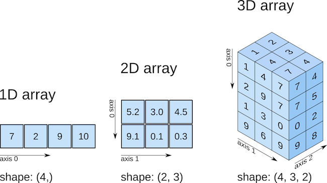
Fig. 3.2 A graphical representation of arrays. You’re probably most familiar with the two-dimensional version, a matrix. Source: Chapter 5 of Python for Data Science#
We need to import the numpy package in order to use narrays. Here’s the syntax for bringing in a package to our code. We’re going to type this at the start of basically all of our code. We are going to use the np part to tell Python where to look for a function/method in the numpy package. This is important, as numpy contains functions like min or max that are also built-in the standard Python. If you just write max(x), Python is going to wonder what max you mean!
You only need to import once per Python session. But, if you restart your Python kernel, you’ll need to run the import again.
import numpy as np
3.2.2. Creating arrays#
We can create our own arrays using data we input ourselves.
my_array = np.array([1, 2, 3, 4, 5])
type(my_array)
numpy.ndarray
We we talk about arrays, we talk about dimensions. A vector just has one dimension, n. A matrix has n rows and k columns. We write this as n x k. You can have an array with as many dimensions as you want. Vectors, matrices, cubes, n-dimensions, etc.
In Python, we talk about the axis of an array. A 1-D array has only one axis, axis-0. A 2-D array, or matrix, has axis-0 (rows) and axis-1 (columns). See the graphic above.
We can also create random numbers. In VS Code, can hold your cursor over the randn part of the function below to see what it is doing. In fact, you can do that on any of the code below! Even the my_random_array object being created by the code.
my_random_array = np.random.randn(2, 3)
my_random_array
array([[-0.15085799, -1.92623955, -1.43108553],
       [-0.64772434,  0.16018298,  0.10133068]])
Notice the [ and ]. Each row gets its own set of brackets, while the entire array is also in brackets.
There are also many built-in methods for creating specific array types.
np.arange(1, 5) # from 1 inclusive to 5 exclusive
array([1, 2, 3, 4])
np.arange(0, 11, 2) # step by 2 from 1 to 11
array([ 0, 2, 4, 6, 8, 10])
np.linspace(0, 10, 5) # 5 equally spaced points between 0 and 10
array([ 0. , 2.5, 5. , 7.5, 10. ])
np.ones((2, 2)) # an array of ones with size 2 x 2
array([[1., 1.],
       [1., 1.]])
Any many others. See Chapter 5 of Python for Data Science.
numpy has several functions for looking at the shapes of our arrays. Let’s create another matrix of random numbers from the standard normal distribution. We will then use .ndim(), .shape(), and .size().
x = np.random.randn(10, 5)
x
array([[-0.68685277,  0.9162152 , -1.7758756 , -1.7767166 , -0.9833378 ],
       [-1.01160119, -0.90055593, -0.87097386,  0.81956334, -0.72487347],
       [-0.73194899, -1.47437784,  0.30574121, -0.89996663, -0.22422793],
       [-1.25389739,  1.28907642,  2.03131067,  1.34091606,  0.507005  ],
       [ 0.06397655,  0.43204744, -1.09267458, -0.47840626,  0.37816307],
       [ 0.36363227,  0.35619788, -0.98535774,  1.49420134,  0.07003   ],
       [ 0.64900989, -0.0768026 ,  0.57264403, -0.3248653 ,  2.13252671],
       [ 1.35433274, -1.53265103, -0.78293062,  0.25224106,  0.87676959],
       [ 2.20602652, -0.86852158,  0.78090847, -1.18736513, -0.63877504],
       [-2.75165827, -0.38598081, -1.18589433, -1.27658217,  1.05553294]])
x.ndim
2
There are two dimensions, axis-0 and axis-1, rows and columns.
x.shape
(10, 5)
10 elements along axis-0 and 5 along axis-1. For a 2-D array, this corresponds to rows and columns.
x.size
50
There are 10 * 5 = 50 total elements in that array.
3.2.3. Array math#
We’ll start with element-by-element operations. You’ve likely seen these in a math class somewhere. We’ll start by creating a 1-D array of ones. You’d be surprised how often you just need a bunch of ones in linear algebra!
x = np.ones(4)
x
array([1., 1., 1., 1.])
y = x + 1
y
array([2., 2., 2., 2.])
x - y
array([-1., -1., -1., -1.])
Those both make sense. You’re simply adding or subtracting an element from one with the corresponding element from the other. How about multiplication (*), raising to an exponent (**), and division? Same thing!
x * y
array([2., 2., 2., 2.])
x ** y
array([1., 1., 1., 1.])
x / y
array([0.5, 0.5, 0.5, 0.5])
3.2.4. Reshaping and resizing#
You can also reshape your arrays. This means rearranging the different axis. Let’s create 1-D array with 8 elements to play with. We can again see the shape attribute with .shape().
x = np.array([1, 2, 3, 4, 5, 6, 7, 8])

x.shape
(8,)
Let’s use .reshape() to change the dimensions of this array. .reshape() lets you go from, say, 1-D to 2-D, using the same data. We’ll a 2 x 4 2-D array.
x.reshape(2,4)
array([[1, 2, 3, 4],
       [5, 6, 7, 8]])
Note that the resulting array needs to have the same number of elements, so 2 * 4 = 8.
If you’ve taken a math class that deals with matrices, then you’ve seen transposition.
Let’s create an array of random numbers between 0 and 1 using .rand(), different from .randn(), that is a 5 x 2 matrix. Then, we’ll .transpose() the array object. This means that we will flip the rows and columns, such that the first row becomes the first column, the second row becomes the second column, and so on. This will result in a 2 x 5 matrix.
x = np.random.rand(5, 2)
x
array([[0.76300789, 0.01592345],
       [0.22698807, 0.534598  ],
       [0.51275612, 0.41626957],
       [0.70908879, 0.71401538],
       [0.62467146, 0.16161006]])
5 rows and 2 columns. OK, let’s transpose this. We’ll use the .transpose() function.
x.transpose()
array([[0.76300789, 0.22698807, 0.51275612, 0.70908879, 0.62467146],
       [0.01592345, 0.534598  , 0.41626957, 0.71401538, 0.16161006]])
Now we have 2 rows and 5 columns.
See how reshape and transpose are doing different things? We can reshape a 2-D array to make this clearer. How about going from 6 x 2 to 3 x 4? That requires a .reshape(). If we instead use .transpose(), we go from 6 x 2 to 2 x 6. No need to specify any rows or columns with transpose.
x = np.random.rand(6, 2)
x
array([[0.79468631, 0.90618805],
       [0.17731804, 0.52260493],
       [0.03383431, 0.7743164 ],
       [0.83147215, 0.82425247],
       [0.71404254, 0.04485264],
       [0.0993507 , 0.26370596]])
x.reshape(3,4)
array([[0.79468631, 0.90618805, 0.17731804, 0.52260493],
       [0.03383431, 0.7743164 , 0.83147215, 0.82425247],
       [0.71404254, 0.04485264, 0.0993507 , 0.26370596]])
x.transpose()
array([[0.79468631, 0.17731804, 0.03383431, 0.83147215, 0.71404254,
        0.0993507 ],
       [0.90618805, 0.52260493, 0.7743164 , 0.82425247, 0.04485264,
        0.26370596]])
Finally, let’s look at .resize(). .reshape() had to have the same number of elements. .resize() does not. Let’s create another random array.
x = np.random.rand(6, 2)
x
array([[0.52472092, 0.23714866],
       [0.58366456, 0.98336204],
       [0.19514394, 0.90128893],
       [0.16318428, 0.71656894],
       [0.51426974, 0.65113506],
       [0.55677245, 0.4407399 ]])
Let’s pick out the first row and then just the first two columns from that.
np.resize(x,(1,2))
array([[0.52472092, 0.23714866]])
Or, how about we make this array bigger? This will add six rows, But, with what numbers? It just repeats the numbers from above to fill in the additional 12 items (6 rows and 2 columns).
np.resize(x,(12,2))
array([[0.52472092, 0.23714866],
       [0.58366456, 0.98336204],
       [0.19514394, 0.90128893],
       [0.16318428, 0.71656894],
       [0.51426974, 0.65113506],
       [0.55677245, 0.4407399 ],
       [0.52472092, 0.23714866],
       [0.58366456, 0.98336204],
       [0.19514394, 0.90128893],
       [0.16318428, 0.71656894],
       [0.51426974, 0.65113506],
       [0.55677245, 0.4407399 ]])
Why do we need to do any of this? Matrix math sometimes requires our data to be in a certain shape.
But, wait… I just wrote my code differently. There’s an x inside the .resize(), rather than just writing x.resize()! And, why are there parentheses around the dimensions? What’s going on?
3.2.4.1. An aside: Functions, methods and objects#
Let’s look at two lines of code from above.
x = np.random.rand(6, 2)
x
array([[0.54868142, 0.29810949],
       [0.71307155, 0.93187129],
       [0.01287844, 0.74263204],
       [0.25100509, 0.92768183],
       [0.36549182, 0.2792388 ],
       [0.10534503, 0.03193589]])
This code is saying: Use the function .rand() from the collection of .random() functions found in the numpy package, which we have abbreviated as np.. This creates a new object called x that is a narray, or numpy array.
Objects are things. Like an array that stores our data. Objects come with methods that let us do things to them. They also come with attributes that let us learn more about them.
x.shape() gets the shape attribute of x.
x.reshape() calls the .reshape() method on object x.
We’ll do a bit more on this later, but I wanted to point out why the code sometimes has np., sometimes has x., and sometimes has x = . Note that you could use a method on an object and then save the result, even over the original object.
x.reshape(3,4)
array([[0.54868142, 0.29810949, 0.71307155, 0.93187129],
       [0.01287844, 0.74263204, 0.25100509, 0.92768183],
       [0.36549182, 0.2792388 , 0.10534503, 0.03193589]])
I could have also written the code another way, which let’s us see the np.. I am including x as an argument to my method. I then have to put () around my new dimensions. This creates a tuple for our dimensions.
np.reshape(x, (3, 4))
array([[0.54868142, 0.29810949, 0.71307155, 0.93187129],
       [0.01287844, 0.74263204, 0.25100509, 0.92768183],
       [0.36549182, 0.2792388 , 0.10534503, 0.03193589]])
Why do it this way? It lets us use the np. pre-fix, which means that Python won’t get confused. For example there’s a np.resize() method and a regular .resize() method. You also need the np. pre-fix in order to be able to put your cursor over the code to get help in VS Code.
x.resize(1, 2)
---------------------------------------------------------------------------
ValueError                                Traceback (most recent call last)
Input In [31], in <cell line: 1>()
----> 1 x.resize(1, 2)

ValueError: cannot resize an array that references or is referenced
by another array in this way.
Use the np.resize function or refcheck=False
See the error message? It is telling us to use the np.resize() function.
np.resize(x, (1,2))
array([[0.91298579, 0.41171994]])
Much better!
You’ll see code written a variety of ways when looking for help online or looking at different books. While this stuff can be confusing at first, it’s helpful to kind of understand what’s going on, so that you can see the subtle differences in syntax and why they matter.
3.2.5. Indexing and slicing#
We’ve seen indexing and slicing already. Let’s look at how we can pull a particular number, row, or column out of an array. There are three particular pieces of syntax to pay attention to: we are using square brackets with arrays [], use are using a comma , to separate the different axis (e.g. rows and columns in a two-dimensional array), and we are using a colon : to slice and get back certain parts of the array.
Let’s create a simple 1-D array to start, the numbers 0 - 9. Remember how Python starts indexing at 0?
x = np.arange(10)
x
array([0, 1, 2, 3, 4, 5, 6, 7, 8, 9])
We can then pull just pieces of that array. Note that we’re using brackets and not parentheses now. Item 3 is the 4th number when you have zero indexing.
x[3]
3
Let’s slice. What if wanted to start on 2 (the third item in the array) and then get everything else after that?
x[2:] # Starting on the third item
array([2, 3, 4, 5, 6, 7, 8, 9])
How about just items 0, 1, and 2?
x[:3] # Up until the 4th item, exclusive.
array([0, 1, 2])
We can select something in the middle too.
x[2:5] # Start on the third item, go up until the 6th item, exclusive.
array([2, 3, 4])
And we can even start from the end of the array when selecting items.
x[-1] # Start counting backwards
9
We do similar things for 2-D arrays. Let’s create a 4 x 6 matrix out of random integers from 0 to 9 (0 to 10, exclusive).
x = np.random.randint(10, size=(4, 6))
x
array([[6, 2, 5, 0, 7, 1],
       [3, 4, 2, 9, 0, 8],
       [9, 6, 0, 6, 6, 8],
       [0, 0, 2, 4, 3, 5]])
We can then pick out the row x column that we want. Using [3,4] gets us the 4th row and the 5th column, since, again, we have zero indexing. We need to start just referring to these as the 3rd row and 4th column and assuming that we start at 0.
x[3,4]
3
We can pick out just the 3rd row. Now, notice how I’m using , and :. The 3 means 3rd row, where we start counting from 0. The , separates our axis, so we have rows,columns. The : is telling Python to slice all of the columns. This way, we’ll get each element of the 3rd row.
x[3,:]
array([0, 0, 2, 4, 3, 5])
We can also pick out just the 4th column using : and , together. This means choose all rows, just the 4th column.
x[:,4]
array([7, 0, 6, 3])
We can select multiple rows and columns, also using : and , together.
x[0:2,:] # Choose the first two rows.
array([[6, 2, 5, 0, 7, 1],
       [3, 4, 2, 9, 0, 8]])
You could have also written that like this. If you don’t put the ,:, Python will assume that you want all of the columns.
x[0:2] # Choose the first two rows.
array([[6, 2, 5, 0, 7, 1],
       [3, 4, 2, 9, 0, 8]])
How about the first two columns? The first : means “all rows”. Then, we separate the rows and columns with ,. Finally, we select the two columns with 0:2.
x[:,0:2]
array([[6, 2],
       [3, 4],
       [9, 6],
       [0, 0]])
Notice how you do need the :, to get all of the rows.
You can also get a piece of the array, not just whole rows and columns.
x[1:3,2:4]
array([[2, 9],
       [0, 6]])
Finally, you can change a number in an array.
x[1,1] = 1000
x
array([[   6,    2,    5,    0,    7,    1],
       [   3, 1000,    2,    9,    0,    8],
       [   9,    6,    0,    6,    6,    8],
       [   0,    0,    2,    4,    3,    5]])
3.2.6. Vectorization#
Vectorization let’s us avoid slow, inefficient loops. Let’s look at example.
array = np.array(range(1000000))
for i, element in enumerate(array):
    array[i] = element ** 2
array = np.array(range(1000000))
array **= 2
The two code blocks above do the exact same thing. They create an array with 1,000,000 numbers, from 1 to 1,000,000. Then, the square each of these. The second code block is 4x faster though!
The first block is a for loop. For each element (number) in the array, that that element and square it.
The second block is vectorized. Python is doing everything at once, in a sense. The **= means take each number in the array and square it. It is a short-cut way to write the loop, but, even better than that, it is faster to run.
By the way, you’ll see the “operation”= thing a lot in code. It means take the thing on the left-hand side, do the operation, in this case “**2”, or square the number, and replace the original array with all of the squared terms. Here’s another example using addition. You can do the same thing with subtraction.
x = 10
x += 1
x
11
We can compare the two methods from above directly. We’ll just do five numbers here, so that the comparison doesn’t take forever.
# loop method
array = np.array(range(5))
time_loop = %timeit -q -o -r 3 for i, element in enumerate(array): array[i] = element ** 2
# vectorized method
array = np.array(range(5))
time_vec = %timeit -q -o -r 3 array ** 2
print(f"Vectorized operation is {time_loop.average / time_vec.average:.2f}x faster than looping here.")
Vectorized operation is 3.63x faster than looping here.
3.2.7. Broadcasting#
We’ll end with broadcasting. Arrays of different dimensions can’t be directly used in arithmetic, element-by-element, operations. For example, let’s create two arrays of different sizes and try adding them together.
a = np.ones((2, 2))
b = np.ones((3, 3))
a + b
---------------------------------------------------------------------------
ValueError                                Traceback (most recent call last)
/var/folders/sm/f4lq92s11392x68kwf0scq3w0000gn/T/ipykernel_82966/2577290910.py in <module>
      1 a = np.ones((2, 2))
      2 b = np.ones((3, 3))
----> 3 a + b

ValueError: operands could not be broadcast together with shapes (2,2) (3,3)
We can’t add a 2 x 2 matrix to a 3 x 3 matrix. It just doesn’t work! So, we need some rules for doing element-by-element operations on our arrays.
Let’s create a 1-D array of prices for three different products: \(10, \)15, and $20. 1-D arrays can be confusing, as they can actually have several different types of shapes.
price = np.array([10, 15, 20])
price
array([10, 15, 20])
Let’s also create an array of quantity sold for the three products. They need to be in the same order as the prices above.
sales = np.array([100, 150, 200])
sales
array([100, 150, 200])
We can multiply the two matrices together to get total revenue by product.
sales * price
array([1000, 2250, 4000])
We can also do something called the dot product using np.dot(). This takes the first element from price and multiplies it by the first element from sales and then adds this to the second item from price times the second item from sales, etc. This results in the total revenue across all products.
np.dot(sales, price)
7250
OK, but what if we have three days of sales across the three products. Now, each row is a different product and each column is a different day.
sales = np.array([[100, 120, 130], [150, 110, 125], [200, 150, 190]])
sales
array([[100, 120, 130],
       [150, 110, 125],
       [200, 150, 190]])
Let’s look at our shapes for price and sales.
price.shape # A 1-D array, with 3 numbers along axis-0.
(3,)
sales.shape # A 3-D array, with 3 numbers along each axis.
(3, 3)
Let’s just multiply these together and see what we get.
price * sales
array([[1000, 1800, 2600],
       [1500, 1650, 2500],
       [2000, 2250, 3800]])
This isn’t right! Each row is a different product, so the first row is all the same item with the same price. Each number in the first row needs to be multiplied by 10. The second row by 15. And the third row by 20.
We can use .reshape() to fix this.
price = price.reshape(3,1)
price
array([[10],
       [15],
       [20]])
See how the numbers are going up and down? OK, now let’s np.repeat() price to get all 10’s in the first row, etc. The syntax is saying to repeat each item three times across the first axis (the columns).
price = np.repeat(price, 3, axis = 1)
price
array([[10, 10, 10],
       [15, 15, 15],
       [20, 20, 20]])
Now, let’s try multiplying.
price * sales
array([[1000, 1200, 1300],
       [2250, 1650, 1875],
       [4000, 3000, 3800]])
This looks good! But, there has to be an easier way, right? Yeah. Let’e set up our original prices again and reshape it, all in one step.
price = np.array([10, 15, 20]).reshape(3,1)
price
array([[10],
       [15],
       [20]])
See how we can “chain” functions and methods together? This creates the object, uses a method, and saves it, all in one line. OK, now just multiply.
price * sales
array([[1000, 1200, 1300],
       [2250, 1650, 1875],
       [4000, 3000, 3800]])
Python is broadcasting, which means that it is doing that .repeat() for us to get the multiplication to work out. We now have the correct revenue for each product by day!
We’ll go over matrix multiplication in Python more when we get to some portfolio mathematics and using SciPy.