2.6. Google Colab

Google Colab is another way to create Jupyter notebooks, denoted by that .ipynb file extension, in your browser.

Why use Google Colab? I think the platform is nicer than the other browser-based Jupyter notebook platform that comes with Anaconda. In the next chapter, I’ll discuss the full-fledged developer environment VS Code, that lets you add numerous extensions, access your terminal (command line), and code in multiple languages. You can use any of the platforms in this class, though I’ll tend to use VS Code in my examples.

To open up a Jupyter Notebook in Google Colab, simply go to the web page. You’ll see the initial window below.

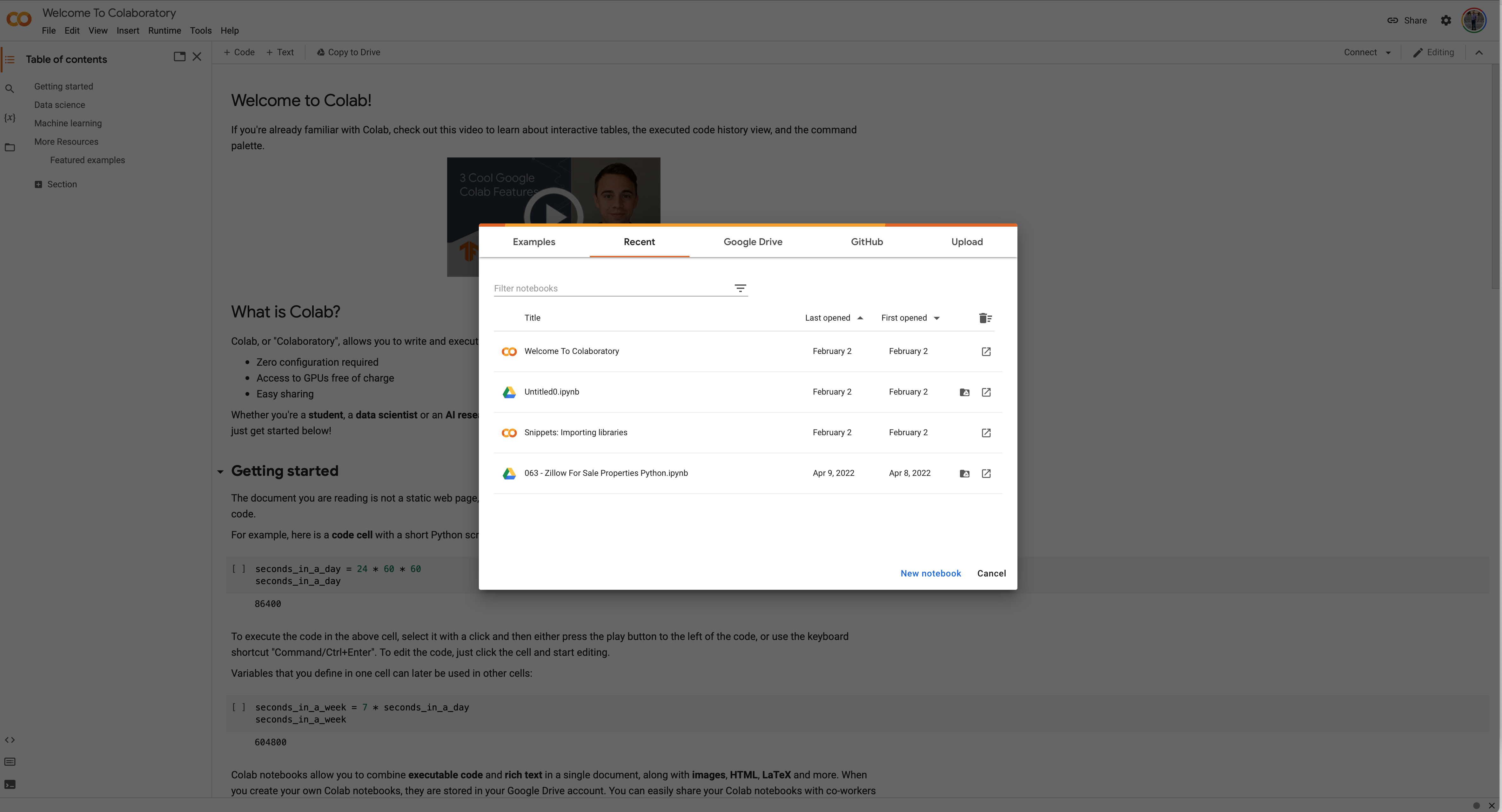
Fig. 2.27 The initial welcome screen for Google Colab. Your notebooks are stored in Google Drive and can be shared. You can also hit cancel and access the Welcome to Colab tutorial.

You can create a new notebook, open one that’s been saved to your Google Drive, or access your notebooks on your GitHub account, if you have one. You don’t need one for this class, but if you’re a data science, analytics, computer science major, you should have a GitHub account and learn to use git to organize and share code.

You can create a folder for this class on Google Drive in order to stay organized.

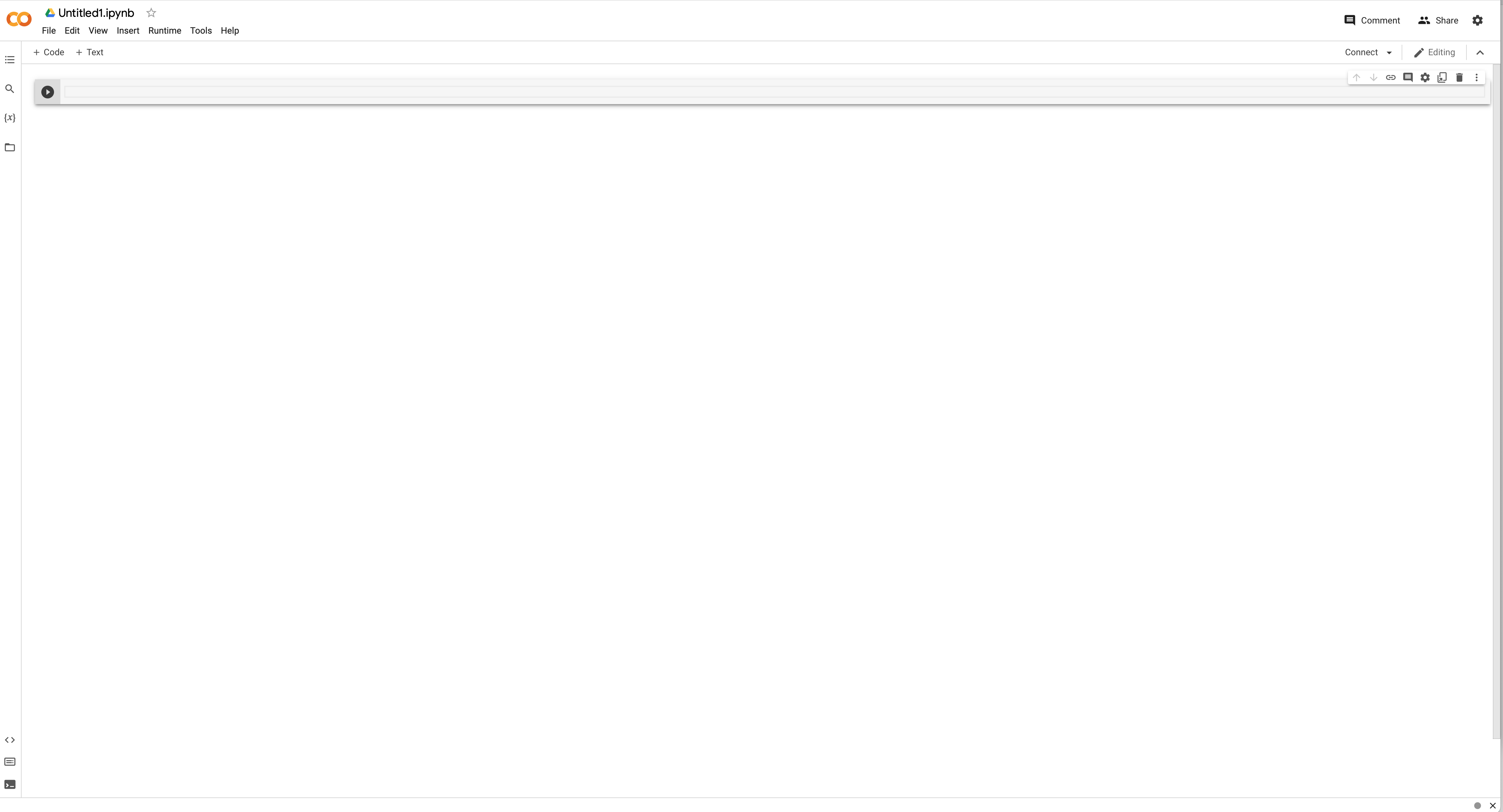
Fig. 2.28 The Google Colab Jupyter notebook looks like any other Jupyter notebook.

If you create a new notebook, you’ll open a new file in your browser called Untitled1.ipynb. You’ll see the + buttons to added a code cell or a Markdown text cell. Notice that with the text cell, you’ll also get some “point and click” options for formatting. You can still use Markdown, though, as is typical in these notebooks. You’ll also see the preview of what the text cell will look like on the right. I discuss Markdown later on in this chapter.

On the top-left, you’ll find four icons. The first is the Table of Contents. Jupyter notebooks understand your headers and sub-headers and will create a table of contents for you that you can use to navigate your document. The magnify glass lets you search your notebook. The bracket x is the variable explorer. You’ll be able to see what variables and data types you’ve created in your code. Finally, the folder lets you see files in your Google Drive, including any data that you might have.

Under the File menu at the top, you can create a new notebook, save your notebook to Google Drive, and, crucially, download the .ipynb file to your local machine, among other actions.

Edit, View, and Insert have the usual set of features.

The Runtime menu lets you run your code all at once, run just certain cells, and restart your runtime (kernel). The latter clears out your memory and lets you start over. As I mention in the problem sets, it’s a good idea to do this when you’re done and try running your code from top to bottom.

You can find and set keyboard shortcuts under Tools. And, of course there is a Help menu.

The bottom-left has three icons. The <> brings up helpful code snippets. The keyboard icon opens a command pallette, similar to the one you’ll see in VS Code. The command prompt icon is to sign up to Colab pro.

All of this is happening in the cloud, on a remote computer. You’ll see how much Google Drive space you’re taking up in the bottom-left. The Ram and Disk settings in the upper-right tell you how much memory you’re taking up. When you load data, that goes into memory.

Finally, you can also check out this set of YouTube videos on using Google Colab.