
pandas#
Now that we know how to get our data in, let’s look a little more at pandas and what it can do. To do this, let’s bring in some data from Zillow.
The data frame we will be working with contains data from Zillow.com, the housing web site, on the number of homes, the median value of homes, etc. at-risk for flooding due to rising sea levels.
You can find many different Zillow data sets here. The “uw” here stands for “under water” in a very literal sense. I first thought they were talking about mortgages!
As mentioned, take a look at Chapter 5 of Python for Data Analysis for an introduction to pandas.
Tip
AI is your pandas syntax partner. There are many ways to select, filter, and transform data in pandas. When you’re stuck, describe what you want in plain English: “I want to keep only rows where the state is North Carolina and the region type is MSA.” Claude will give you the exact syntax - often showing multiple approaches so you can pick the one that makes the most sense to you.
import numpy as np
import pandas as pd

uw = pd.read_csv('https://github.com/aaiken1/fin-data-analysis-python/raw/main/data/zestimatesAndCutoffs_byGeo_uw_2017-10-10_forDataPage.csv')
We are going to use read_csv to get this data off of my Github page. pandas also comes with read_excel, read_json, read_html, and other ways to get formatted data into Python.
Looking at our data#
Let’s peak at this data. You can do that below, or using the .info method. We’ll get variable names, the number of non-missing (null) observations, and the type of data. One number variable, UWHomes_Tier2, got brought in as an integer, rather than a float. When you look at the data below, notice how that one column doesn’t have a .0 on any of the numbers. Integers can’t have decimal places.
uw.info()
<class 'pandas.core.frame.DataFrame'>
RangeIndex: 2610 entries, 0 to 2609
Data columns (total 24 columns):
 #   Column                        Non-Null Count  Dtype
---  ------                        --------------  -----
 0   RegionType                    2610 non-null   object
 1   RegionName                    2610 non-null   object
 2   StateName                     2609 non-null   object
 3   MSAName                       1071 non-null   object
 4   AllHomes_Tier1                2610 non-null   float64
 5   AllHomes_Tier2                2610 non-null   float64
 6   AllHomes_Tier3                2610 non-null   float64
 7   AllHomes_AllTiers             2610 non-null   float64
 8   UWHomes_Tier1                 2610 non-null   float64
 9   UWHomes_Tier2                 2610 non-null   int64
 10  UWHomes_Tier3                 2610 non-null   float64
 11  UWHomes_AllTiers              2610 non-null   float64
 12  UWHomes_TotalValue_Tier1      2610 non-null   float64
 13  UWHomes_TotalValue_Tier2      2610 non-null   float64
 14  UWHomes_TotalValue_Tier3      2610 non-null   float64
 15  UWHomes_TotalValue_AllTiers   2610 non-null   float64
 16  UWHomes_MedianValue_AllTiers  2610 non-null   float64
 17  AllHomes_Tier1_ShareUW        2610 non-null   float64
 18  AllHomes_Tier2_ShareUW        2610 non-null   float64
 19  AllHomes_Tier3_ShareUW        2610 non-null   float64
 20  AllHomes_AllTiers_ShareUW     2610 non-null   float64
 21  UWHomes_ShareInTier1          2610 non-null   float64
 22  UWHomes_ShareInTier2          2610 non-null   float64
 23  UWHomes_ShareInTier3          2610 non-null   float64
dtypes: float64(19), int64(1), object(4)
memory usage: 489.5+ KB
Just to show you, I’m going to reimport that data, but force that one variable to also come in as the same variable type. I don’t want anything unexpected to happen, so let’s get all numerics as floats. Notice how I do this – I give the column, or variable name, and the data type I want. I’m using a particular type of float type that comes with the numpy package.
uw = pd.read_csv('https://github.com/aaiken1/fin-data-analysis-python/raw/main/data/zestimatesAndCutoffs_byGeo_uw_2017-10-10_forDataPage.csv', dtype = {'UWHomes_Tier2':np.float64})
uw.info()
<class 'pandas.core.frame.DataFrame'>
RangeIndex: 2610 entries, 0 to 2609
Data columns (total 24 columns):
 #   Column                        Non-Null Count  Dtype
---  ------                        --------------  -----
 0   RegionType                    2610 non-null   object
 1   RegionName                    2610 non-null   object
 2   StateName                     2609 non-null   object
 3   MSAName                       1071 non-null   object
 4   AllHomes_Tier1                2610 non-null   float64
 5   AllHomes_Tier2                2610 non-null   float64
 6   AllHomes_Tier3                2610 non-null   float64
 7   AllHomes_AllTiers             2610 non-null   float64
 8   UWHomes_Tier1                 2610 non-null   float64
 9   UWHomes_Tier2                 2610 non-null   float64
 10  UWHomes_Tier3                 2610 non-null   float64
 11  UWHomes_AllTiers              2610 non-null   float64
 12  UWHomes_TotalValue_Tier1      2610 non-null   float64
 13  UWHomes_TotalValue_Tier2      2610 non-null   float64
 14  UWHomes_TotalValue_Tier3      2610 non-null   float64
 15  UWHomes_TotalValue_AllTiers   2610 non-null   float64
 16  UWHomes_MedianValue_AllTiers  2610 non-null   float64
 17  AllHomes_Tier1_ShareUW        2610 non-null   float64
 18  AllHomes_Tier2_ShareUW        2610 non-null   float64
 19  AllHomes_Tier3_ShareUW        2610 non-null   float64
 20  AllHomes_AllTiers_ShareUW     2610 non-null   float64
 21  UWHomes_ShareInTier1          2610 non-null   float64
 22  UWHomes_ShareInTier2          2610 non-null   float64
 23  UWHomes_ShareInTier3          2610 non-null   float64
dtypes: float64(20), object(4)
memory usage: 489.5+ KB
OK, that seems better. All of these functions that we’re using have many different options. The only way to learn about them is to play around, read help documents, and search online for solutions to our problems.
There’s a concept in data analysis called tidy data. The characteristics of tidy data are:
Each variable forms a column.
Each observation forms a row.
Each type of observational unit forms a table.
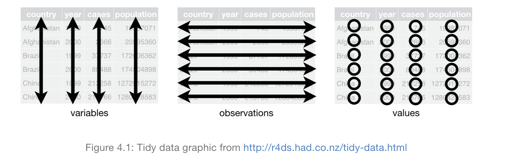
Fig. 37 Tidy data.#
The first thing to note about this data is that there are several tiers. Some numbers are at the national level, some at the region, some at the state, and some at the MSA. Tidy data refers to one row, one observation, across different variables (columns) and, possibly, across time. When you have multiple observations of the same firm, state, person, etc. over time, we call that panel data. Panel data is tidy too.
Note that some RegionTypes (e.g. Nation, State) are actually summaries of other rows. This is bit confusing and we need to be mindful of this different levels when using the data.
Before we get to that, just a few more methods to look at the data.
First, let’s look at the first five rows.
uw.head()
| RegionType | RegionName | StateName | MSAName | AllHomes_Tier1 | AllHomes_Tier2 | AllHomes_Tier3 | AllHomes_AllTiers | UWHomes_Tier1 | UWHomes_Tier2 | ... | UWHomes_TotalValue_Tier3 | UWHomes_TotalValue_AllTiers | UWHomes_MedianValue_AllTiers | AllHomes_Tier1_ShareUW | AllHomes_Tier2_ShareUW | AllHomes_Tier3_ShareUW | AllHomes_AllTiers_ShareUW | UWHomes_ShareInTier1 | UWHomes_ShareInTier2 | UWHomes_ShareInTier3 | |
|---|---|---|---|---|---|---|---|---|---|---|---|---|---|---|---|---|---|---|---|---|---|
| 0 | Nation | United States | NaN | NaN | 35461549.0 | 35452941.0 | 35484532.0 | 106399022.0 | 594672.0 | 542681.0 | ... | 5.974490e+11 | 9.159540e+11 | 310306.0 | 0.016769 | 0.015307 | 0.020458 | 0.017512 | 0.319149 | 0.291246 | 0.389605 |
| 1 | State | Alabama | Alabama | NaN | 546670.0 | 520247.0 | 491300.0 | 1558217.0 | 2890.0 | 2766.0 | ... | 2.583039e+09 | 3.578203e+09 | 270254.0 | 0.005287 | 0.005317 | 0.010271 | 0.006868 | 0.270043 | 0.258456 | 0.471501 |
| 2 | State | California | California | NaN | 3060171.0 | 3076238.0 | 3169584.0 | 9305993.0 | 8090.0 | 14266.0 | ... | 2.666638e+10 | 4.449536e+10 | 860373.0 | 0.002644 | 0.004637 | 0.005611 | 0.004313 | 0.201550 | 0.355415 | 0.443035 |
| 3 | State | Connecticut | Connecticut | NaN | 333904.0 | 334688.0 | 336254.0 | 1004846.0 | 4434.0 | 3807.0 | ... | 8.689480e+09 | 1.152170e+10 | 442036.0 | 0.013279 | 0.011375 | 0.021677 | 0.015455 | 0.285512 | 0.245138 | 0.469350 |
| 4 | State | Delaware | Delaware | NaN | 102983.0 | 127573.0 | 127983.0 | 358539.0 | 4105.0 | 2574.0 | ... | 1.498013e+09 | 2.801847e+09 | 241344.5 | 0.039861 | 0.020177 | 0.025675 | 0.027793 | 0.411942 | 0.258304 | 0.329754 |
5 rows × 24 columns
NaN is how pandas shows missing values. So, that first row is RegionType == 'Nation' and RegionName == 'UnitedStates'. StateName and MSAName are undefined, since this row is all of the data added up. We usually don’t want to have summary statistics in the same DataFrame as underlying data! What a mess!
We can also look at the last five rows.
uw.tail()
| RegionType | RegionName | StateName | MSAName | AllHomes_Tier1 | AllHomes_Tier2 | AllHomes_Tier3 | AllHomes_AllTiers | UWHomes_Tier1 | UWHomes_Tier2 | ... | UWHomes_TotalValue_Tier3 | UWHomes_TotalValue_AllTiers | UWHomes_MedianValue_AllTiers | AllHomes_Tier1_ShareUW | AllHomes_Tier2_ShareUW | AllHomes_Tier3_ShareUW | AllHomes_AllTiers_ShareUW | UWHomes_ShareInTier1 | UWHomes_ShareInTier2 | UWHomes_ShareInTier3 | |
|---|---|---|---|---|---|---|---|---|---|---|---|---|---|---|---|---|---|---|---|---|---|
| 2605 | Zip | 98592 | Washington | NaN | 464.0 | 470.0 | 493.0 | 1427.0 | 8.0 | 29.0 | ... | 73407109.0 | 82715412.0 | 436490.5 | 0.017241 | 0.061702 | 0.273834 | 0.120533 | 0.046512 | 0.168605 | 0.784884 |
| 2606 | Zip | 98595 | Washington | NaN | 558.0 | 571.0 | 598.0 | 1727.0 | 119.0 | 104.0 | ... | 13761194.0 | 40365702.0 | 131441.0 | 0.213262 | 0.182137 | 0.095318 | 0.162131 | 0.425000 | 0.371429 | 0.203571 |
| 2607 | Zip | 98612 | Washington | NaN | 365.0 | 376.0 | 409.0 | 1150.0 | 91.0 | 79.0 | ... | 14406737.0 | 50284001.0 | 230495.0 | 0.249315 | 0.210106 | 0.092910 | 0.180870 | 0.437500 | 0.379808 | 0.182692 |
| 2608 | Zip | 32081 | Florida | NaN | 1318.0 | 1328.0 | 1350.0 | 3996.0 | 91.0 | 42.0 | ... | 91112117.0 | 132505542.0 | 385196.0 | 0.069044 | 0.031627 | 0.097778 | 0.066316 | 0.343396 | 0.158491 | 0.498113 |
| 2609 | Zip | 33578 | Florida | NaN | 5975.0 | 4537.0 | 3232.0 | 13744.0 | 8.0 | 6.0 | ... | 56852018.0 | 59115506.0 | 363355.0 | 0.001339 | 0.001322 | 0.038366 | 0.010041 | 0.057971 | 0.043478 | 0.898551 |
5 rows × 24 columns
Looking at this data, I think it really has four levels that describe the numbers. The columns RegionType, RegionName, StateName, and MSAName define unique rows of data. Again, note that these values can be missing. For example, row 2606 is Zip, 98595, Washington, but no MSAName. Why? MSA stands for Metropolitan Statistical Area and covers multiple zip codes. This data is not tidy.
Let’s think about the other variable definitions a bit. Zillow places homes into three tiers based on the home’s estimated market value, with Tier3 being the highest value. AllHomes refers to all homes in that tier or across all tiers. UWHomes refers to homes that are at risk for flooding. Note that there are some variables that are counts, some that are dollar values, and others that are percentages.
Finally, when using a Jupyter notebook, you can just put the name of the DataFrame in a cell and run the cell. You’ll get a peak at the DataFrame too. If you’re using a Python script, not a Jupyter notebook, then you have to do things like use print() to get the data to display. The Jupyter notebook does this automatically for us.
uw
| RegionType | RegionName | StateName | MSAName | AllHomes_Tier1 | AllHomes_Tier2 | AllHomes_Tier3 | AllHomes_AllTiers | UWHomes_Tier1 | UWHomes_Tier2 | ... | UWHomes_TotalValue_Tier3 | UWHomes_TotalValue_AllTiers | UWHomes_MedianValue_AllTiers | AllHomes_Tier1_ShareUW | AllHomes_Tier2_ShareUW | AllHomes_Tier3_ShareUW | AllHomes_AllTiers_ShareUW | UWHomes_ShareInTier1 | UWHomes_ShareInTier2 | UWHomes_ShareInTier3 | |
|---|---|---|---|---|---|---|---|---|---|---|---|---|---|---|---|---|---|---|---|---|---|
| 0 | Nation | United States | NaN | NaN | 35461549.0 | 35452941.0 | 35484532.0 | 106399022.0 | 594672.0 | 542681.0 | ... | 5.974490e+11 | 9.159540e+11 | 310306.0 | 0.016769 | 0.015307 | 0.020458 | 0.017512 | 0.319149 | 0.291246 | 0.389605 |
| 1 | State | Alabama | Alabama | NaN | 546670.0 | 520247.0 | 491300.0 | 1558217.0 | 2890.0 | 2766.0 | ... | 2.583039e+09 | 3.578203e+09 | 270254.0 | 0.005287 | 0.005317 | 0.010271 | 0.006868 | 0.270043 | 0.258456 | 0.471501 |
| 2 | State | California | California | NaN | 3060171.0 | 3076238.0 | 3169584.0 | 9305993.0 | 8090.0 | 14266.0 | ... | 2.666638e+10 | 4.449536e+10 | 860373.0 | 0.002644 | 0.004637 | 0.005611 | 0.004313 | 0.201550 | 0.355415 | 0.443035 |
| 3 | State | Connecticut | Connecticut | NaN | 333904.0 | 334688.0 | 336254.0 | 1004846.0 | 4434.0 | 3807.0 | ... | 8.689480e+09 | 1.152170e+10 | 442036.0 | 0.013279 | 0.011375 | 0.021677 | 0.015455 | 0.285512 | 0.245138 | 0.469350 |
| 4 | State | Delaware | Delaware | NaN | 102983.0 | 127573.0 | 127983.0 | 358539.0 | 4105.0 | 2574.0 | ... | 1.498013e+09 | 2.801847e+09 | 241344.5 | 0.039861 | 0.020177 | 0.025675 | 0.027793 | 0.411942 | 0.258304 | 0.329754 |
| ... | ... | ... | ... | ... | ... | ... | ... | ... | ... | ... | ... | ... | ... | ... | ... | ... | ... | ... | ... | ... | ... |
| 2605 | Zip | 98592 | Washington | NaN | 464.0 | 470.0 | 493.0 | 1427.0 | 8.0 | 29.0 | ... | 7.340711e+07 | 8.271541e+07 | 436490.5 | 0.017241 | 0.061702 | 0.273834 | 0.120533 | 0.046512 | 0.168605 | 0.784884 |
| 2606 | Zip | 98595 | Washington | NaN | 558.0 | 571.0 | 598.0 | 1727.0 | 119.0 | 104.0 | ... | 1.376119e+07 | 4.036570e+07 | 131441.0 | 0.213262 | 0.182137 | 0.095318 | 0.162131 | 0.425000 | 0.371429 | 0.203571 |
| 2607 | Zip | 98612 | Washington | NaN | 365.0 | 376.0 | 409.0 | 1150.0 | 91.0 | 79.0 | ... | 1.440674e+07 | 5.028400e+07 | 230495.0 | 0.249315 | 0.210106 | 0.092910 | 0.180870 | 0.437500 | 0.379808 | 0.182692 |
| 2608 | Zip | 32081 | Florida | NaN | 1318.0 | 1328.0 | 1350.0 | 3996.0 | 91.0 | 42.0 | ... | 9.111212e+07 | 1.325055e+08 | 385196.0 | 0.069044 | 0.031627 | 0.097778 | 0.066316 | 0.343396 | 0.158491 | 0.498113 |
| 2609 | Zip | 33578 | Florida | NaN | 5975.0 | 4537.0 | 3232.0 | 13744.0 | 8.0 | 6.0 | ... | 5.685202e+07 | 5.911551e+07 | 363355.0 | 0.001339 | 0.001322 | 0.038366 | 0.010041 | 0.057971 | 0.043478 | 0.898551 |
2610 rows × 24 columns
Saving our work#
You’re going to see syntax like:
df = df.some_stuff
This means that our work is getting assigned to something in memory. This is kind of like saving our work. In this case, I’m replacing my original DataFrame df with another DataFrame, also called df. I could have changed the name of the DataFrame.
You’ll also see the inplace = True argument in some functions. This means that the old DataFrame will get overwritten automatically by whatever you just did.
Note
If you don’t assign your work to a placeholder in memory, then the Jupyter Notebook will show you a result, but it doesn’t get reflected in the DataFrame. So, if you try use what you just did, Python won’t know about it!
Selecting our data#
You access columns in pandas like this, using [] and ''. A column is a variable in our data set.
uw['RegionType']
0       Nation
1        State
2        State
3        State
4        State
         ...
2605       Zip
2606       Zip
2607       Zip
2608       Zip
2609       Zip
Name: RegionType, Length: 2610, dtype: object
But, wait, you can also do this! But, only if the variable name doesn’t have spaces. The method with ['NAME'] is more general and can handle variable names with spaces, like ['Var Name'].
uw.RegionType
0       Nation
1        State
2        State
3        State
4        State
         ...
2605       Zip
2606       Zip
2607       Zip
2608       Zip
2609       Zip
Name: RegionType, Length: 2610, dtype: object
Notice how as you’re typing, VS Code and Google Colab are trying to autocomplete for you? Helpful!
You can also do multiple columns. Use a , to separate the column names in []. There are now two pairs of [].
uw[['RegionType', 'RegionName', 'UWHomes_Tier2']]
| RegionType | RegionName | UWHomes_Tier2 | |
|---|---|---|---|
| 0 | Nation | United States | 542681.0 |
| 1 | State | Alabama | 2766.0 |
| 2 | State | California | 14266.0 |
| 3 | State | Connecticut | 3807.0 |
| 4 | State | Delaware | 2574.0 |
| ... | ... | ... | ... |
| 2605 | Zip | 98592 | 29.0 |
| 2606 | Zip | 98595 | 104.0 |
| 2607 | Zip | 98612 | 79.0 |
| 2608 | Zip | 32081 | 42.0 |
| 2609 | Zip | 33578 | 6.0 |
2610 rows × 3 columns
You can save the new DataFrame with just those three columns if you want to use it elsewhere.
uw_only_three_columns = uw[['RegionType', 'RegionName', 'UWHomes_Tier2']]
uw_only_three_columns
| RegionType | RegionName | UWHomes_Tier2 | |
|---|---|---|---|
| 0 | Nation | United States | 542681.0 |
| 1 | State | Alabama | 2766.0 |
| 2 | State | California | 14266.0 |
| 3 | State | Connecticut | 3807.0 |
| 4 | State | Delaware | 2574.0 |
| ... | ... | ... | ... |
| 2605 | Zip | 98592 | 29.0 |
| 2606 | Zip | 98595 | 104.0 |
| 2607 | Zip | 98612 | 79.0 |
| 2608 | Zip | 32081 | 42.0 |
| 2609 | Zip | 33578 | 6.0 |
2610 rows × 3 columns
We are using a list - the column names are in a list defined using []. This is why we had to go through lists earlier - they show up a lot.
You can also pull out just certain rows. We used head and tail above to do this in an “automated” way.
uw[0:10]
| RegionType | RegionName | StateName | MSAName | AllHomes_Tier1 | AllHomes_Tier2 | AllHomes_Tier3 | AllHomes_AllTiers | UWHomes_Tier1 | UWHomes_Tier2 | ... | UWHomes_TotalValue_Tier3 | UWHomes_TotalValue_AllTiers | UWHomes_MedianValue_AllTiers | AllHomes_Tier1_ShareUW | AllHomes_Tier2_ShareUW | AllHomes_Tier3_ShareUW | AllHomes_AllTiers_ShareUW | UWHomes_ShareInTier1 | UWHomes_ShareInTier2 | UWHomes_ShareInTier3 | |
|---|---|---|---|---|---|---|---|---|---|---|---|---|---|---|---|---|---|---|---|---|---|
| 0 | Nation | United States | NaN | NaN | 35461549.0 | 35452941.0 | 35484532.0 | 106399022.0 | 594672.0 | 542681.0 | ... | 5.974490e+11 | 9.159540e+11 | 310306.0 | 0.016769 | 0.015307 | 0.020458 | 0.017512 | 0.319149 | 0.291246 | 0.389605 |
| 1 | State | Alabama | Alabama | NaN | 546670.0 | 520247.0 | 491300.0 | 1558217.0 | 2890.0 | 2766.0 | ... | 2.583039e+09 | 3.578203e+09 | 270254.0 | 0.005287 | 0.005317 | 0.010271 | 0.006868 | 0.270043 | 0.258456 | 0.471501 |
| 2 | State | California | California | NaN | 3060171.0 | 3076238.0 | 3169584.0 | 9305993.0 | 8090.0 | 14266.0 | ... | 2.666638e+10 | 4.449536e+10 | 860373.0 | 0.002644 | 0.004637 | 0.005611 | 0.004313 | 0.201550 | 0.355415 | 0.443035 |
| 3 | State | Connecticut | Connecticut | NaN | 333904.0 | 334688.0 | 336254.0 | 1004846.0 | 4434.0 | 3807.0 | ... | 8.689480e+09 | 1.152170e+10 | 442036.0 | 0.013279 | 0.011375 | 0.021677 | 0.015455 | 0.285512 | 0.245138 | 0.469350 |
| 4 | State | Delaware | Delaware | NaN | 102983.0 | 127573.0 | 127983.0 | 358539.0 | 4105.0 | 2574.0 | ... | 1.498013e+09 | 2.801847e+09 | 241344.5 | 0.039861 | 0.020177 | 0.025675 | 0.027793 | 0.411942 | 0.258304 | 0.329754 |
| 5 | State | Florida | Florida | NaN | 2391491.0 | 2435575.0 | 2456637.0 | 7283703.0 | 313090.0 | 263276.0 | ... | 2.782440e+11 | 4.163480e+11 | 276690.0 | 0.130918 | 0.108096 | 0.135070 | 0.124687 | 0.344743 | 0.289893 | 0.365364 |
| 6 | State | Georgia | Georgia | NaN | 1003890.0 | 986416.0 | 920843.0 | 2911149.0 | 5433.0 | 6904.0 | ... | 6.102691e+09 | 9.565510e+09 | 295405.0 | 0.005412 | 0.006999 | 0.010676 | 0.007615 | 0.245083 | 0.311440 | 0.443477 |
| 7 | State | Hawaii | Hawaii | NaN | 132718.0 | 132760.0 | 139397.0 | 404875.0 | 16716.0 | 12536.0 | ... | 1.134778e+10 | 2.516682e+10 | 500666.0 | 0.125951 | 0.094426 | 0.051658 | 0.090035 | 0.458563 | 0.343895 | 0.197542 |
| 8 | State | Louisiana | Louisiana | NaN | 439606.0 | 424665.0 | 417773.0 | 1282044.0 | 25678.0 | 23280.0 | ... | 6.755054e+09 | 1.309180e+10 | 149888.0 | 0.058411 | 0.054820 | 0.060408 | 0.057872 | 0.346088 | 0.313768 | 0.340144 |
| 9 | State | Massachusetts | Massachusetts | NaN | 610378.0 | 611776.0 | 611920.0 | 1834074.0 | 16830.0 | 16491.0 | ... | 3.436795e+10 | 4.988792e+10 | 582126.0 | 0.027573 | 0.026956 | 0.040749 | 0.031763 | 0.288897 | 0.283078 | 0.428025 |
10 rows × 24 columns
Again, notice how Python starts counting from 0. That 0, 1, 2… shows the current index for this DataFrame. We could change this and will later.
Using loc#
pandas has two location methods: loc and iloc. They are going to let us select parts of our data. The main difference: loc is labelled based and iloc is location based.
Since our columns have labels (our rows do not), we can use loc to specify columns by name. If we created an index for this data, then our rows would have labels. We’ll do that later. Any index for this data will be complicated, since no one column uniquely identifies anything!
You can read more about the two methods here.
We’ll start with loc. Again, our rows don’t have labels or an index, so we can use the number of the row, even with loc. We can pull just the first row of data.
uw.loc[0]
RegionType                              Nation
RegionName                       United States
StateName                                  NaN
MSAName                                    NaN
AllHomes_Tier1                      35461549.0
AllHomes_Tier2                      35452941.0
AllHomes_Tier3                      35484532.0
AllHomes_AllTiers                  106399022.0
UWHomes_Tier1                         594672.0
UWHomes_Tier2                         542681.0
UWHomes_Tier3                         725955.0
UWHomes_AllTiers                     1863308.0
UWHomes_TotalValue_Tier1        122992000000.0
UWHomes_TotalValue_Tier2        195513000000.0
UWHomes_TotalValue_Tier3        597449000000.0
UWHomes_TotalValue_AllTiers     915954000000.0
UWHomes_MedianValue_AllTiers          310306.0
AllHomes_Tier1_ShareUW                0.016769
AllHomes_Tier2_ShareUW                0.015307
AllHomes_Tier3_ShareUW                0.020458
AllHomes_AllTiers_ShareUW             0.017512
UWHomes_ShareInTier1                  0.319149
UWHomes_ShareInTier2                  0.291246
UWHomes_ShareInTier3                  0.389605
Name: 0, dtype: object
That returned a series with just the first row and all of the columns. You can make the output in a Jupyter notebook look a little nicer by turning the series into a DataFrame using to.frame(). Again, this is the first row and all of the column headers, just turned sideways.
uw.loc[0].to_frame()
| 0 | |
|---|---|
| RegionType | Nation |
| RegionName | United States |
| StateName | NaN |
| MSAName | NaN |
| AllHomes_Tier1 | 35461549.0 |
| AllHomes_Tier2 | 35452941.0 |
| AllHomes_Tier3 | 35484532.0 |
| AllHomes_AllTiers | 106399022.0 |
| UWHomes_Tier1 | 594672.0 |
| UWHomes_Tier2 | 542681.0 |
| UWHomes_Tier3 | 725955.0 |
| UWHomes_AllTiers | 1863308.0 |
| UWHomes_TotalValue_Tier1 | 122992000000.0 |
| UWHomes_TotalValue_Tier2 | 195513000000.0 |
| UWHomes_TotalValue_Tier3 | 597449000000.0 |
| UWHomes_TotalValue_AllTiers | 915954000000.0 |
| UWHomes_MedianValue_AllTiers | 310306.0 |
| AllHomes_Tier1_ShareUW | 0.016769 |
| AllHomes_Tier2_ShareUW | 0.015307 |
| AllHomes_Tier3_ShareUW | 0.020458 |
| AllHomes_AllTiers_ShareUW | 0.017512 |
| UWHomes_ShareInTier1 | 0.319149 |
| UWHomes_ShareInTier2 | 0.291246 |
| UWHomes_ShareInTier3 | 0.389605 |
Things look more like what you’d expect if you pull multiple rows. This will also mean that we get a DataFrame and not just a series.
We can pull the first ten rows and just three columns. But, now we are going to use the column names. And - notice how 0:9 actually gets us 0:9! Because we are using loc, we include the last item in the range.
uw.loc[0:9,['RegionType', 'RegionName', 'UWHomes_Tier2']]
| RegionType | RegionName | UWHomes_Tier2 | |
|---|---|---|---|
| 0 | Nation | United States | 542681.0 |
| 1 | State | Alabama | 2766.0 |
| 2 | State | California | 14266.0 |
| 3 | State | Connecticut | 3807.0 |
| 4 | State | Delaware | 2574.0 |
| 5 | State | Florida | 263276.0 |
| 6 | State | Georgia | 6904.0 |
| 7 | State | Hawaii | 12536.0 |
| 8 | State | Louisiana | 23280.0 |
| 9 | State | Massachusetts | 16491.0 |
We could pull all of the columns and rows 0:9 like this.
uw.loc[0:9,:]
| RegionType | RegionName | StateName | MSAName | AllHomes_Tier1 | AllHomes_Tier2 | AllHomes_Tier3 | AllHomes_AllTiers | UWHomes_Tier1 | UWHomes_Tier2 | ... | UWHomes_TotalValue_Tier3 | UWHomes_TotalValue_AllTiers | UWHomes_MedianValue_AllTiers | AllHomes_Tier1_ShareUW | AllHomes_Tier2_ShareUW | AllHomes_Tier3_ShareUW | AllHomes_AllTiers_ShareUW | UWHomes_ShareInTier1 | UWHomes_ShareInTier2 | UWHomes_ShareInTier3 | |
|---|---|---|---|---|---|---|---|---|---|---|---|---|---|---|---|---|---|---|---|---|---|
| 0 | Nation | United States | NaN | NaN | 35461549.0 | 35452941.0 | 35484532.0 | 106399022.0 | 594672.0 | 542681.0 | ... | 5.974490e+11 | 9.159540e+11 | 310306.0 | 0.016769 | 0.015307 | 0.020458 | 0.017512 | 0.319149 | 0.291246 | 0.389605 |
| 1 | State | Alabama | Alabama | NaN | 546670.0 | 520247.0 | 491300.0 | 1558217.0 | 2890.0 | 2766.0 | ... | 2.583039e+09 | 3.578203e+09 | 270254.0 | 0.005287 | 0.005317 | 0.010271 | 0.006868 | 0.270043 | 0.258456 | 0.471501 |
| 2 | State | California | California | NaN | 3060171.0 | 3076238.0 | 3169584.0 | 9305993.0 | 8090.0 | 14266.0 | ... | 2.666638e+10 | 4.449536e+10 | 860373.0 | 0.002644 | 0.004637 | 0.005611 | 0.004313 | 0.201550 | 0.355415 | 0.443035 |
| 3 | State | Connecticut | Connecticut | NaN | 333904.0 | 334688.0 | 336254.0 | 1004846.0 | 4434.0 | 3807.0 | ... | 8.689480e+09 | 1.152170e+10 | 442036.0 | 0.013279 | 0.011375 | 0.021677 | 0.015455 | 0.285512 | 0.245138 | 0.469350 |
| 4 | State | Delaware | Delaware | NaN | 102983.0 | 127573.0 | 127983.0 | 358539.0 | 4105.0 | 2574.0 | ... | 1.498013e+09 | 2.801847e+09 | 241344.5 | 0.039861 | 0.020177 | 0.025675 | 0.027793 | 0.411942 | 0.258304 | 0.329754 |
| 5 | State | Florida | Florida | NaN | 2391491.0 | 2435575.0 | 2456637.0 | 7283703.0 | 313090.0 | 263276.0 | ... | 2.782440e+11 | 4.163480e+11 | 276690.0 | 0.130918 | 0.108096 | 0.135070 | 0.124687 | 0.344743 | 0.289893 | 0.365364 |
| 6 | State | Georgia | Georgia | NaN | 1003890.0 | 986416.0 | 920843.0 | 2911149.0 | 5433.0 | 6904.0 | ... | 6.102691e+09 | 9.565510e+09 | 295405.0 | 0.005412 | 0.006999 | 0.010676 | 0.007615 | 0.245083 | 0.311440 | 0.443477 |
| 7 | State | Hawaii | Hawaii | NaN | 132718.0 | 132760.0 | 139397.0 | 404875.0 | 16716.0 | 12536.0 | ... | 1.134778e+10 | 2.516682e+10 | 500666.0 | 0.125951 | 0.094426 | 0.051658 | 0.090035 | 0.458563 | 0.343895 | 0.197542 |
| 8 | State | Louisiana | Louisiana | NaN | 439606.0 | 424665.0 | 417773.0 | 1282044.0 | 25678.0 | 23280.0 | ... | 6.755054e+09 | 1.309180e+10 | 149888.0 | 0.058411 | 0.054820 | 0.060408 | 0.057872 | 0.346088 | 0.313768 | 0.340144 |
| 9 | State | Massachusetts | Massachusetts | NaN | 610378.0 | 611776.0 | 611920.0 | 1834074.0 | 16830.0 | 16491.0 | ... | 3.436795e+10 | 4.988792e+10 | 582126.0 | 0.027573 | 0.026956 | 0.040749 | 0.031763 | 0.288897 | 0.283078 | 0.428025 |
10 rows × 24 columns
We can pull a range for columns too. Again, notice that the column name range is inclusive of the last column, unlike with slicing by element number.
uw.loc[0:9,'RegionType':'UWHomes_Tier2']
| RegionType | RegionName | StateName | MSAName | AllHomes_Tier1 | AllHomes_Tier2 | AllHomes_Tier3 | AllHomes_AllTiers | UWHomes_Tier1 | UWHomes_Tier2 | |
|---|---|---|---|---|---|---|---|---|---|---|
| 0 | Nation | United States | NaN | NaN | 35461549.0 | 35452941.0 | 35484532.0 | 106399022.0 | 594672.0 | 542681.0 |
| 1 | State | Alabama | Alabama | NaN | 546670.0 | 520247.0 | 491300.0 | 1558217.0 | 2890.0 | 2766.0 |
| 2 | State | California | California | NaN | 3060171.0 | 3076238.0 | 3169584.0 | 9305993.0 | 8090.0 | 14266.0 |
| 3 | State | Connecticut | Connecticut | NaN | 333904.0 | 334688.0 | 336254.0 | 1004846.0 | 4434.0 | 3807.0 |
| 4 | State | Delaware | Delaware | NaN | 102983.0 | 127573.0 | 127983.0 | 358539.0 | 4105.0 | 2574.0 |
| 5 | State | Florida | Florida | NaN | 2391491.0 | 2435575.0 | 2456637.0 | 7283703.0 | 313090.0 | 263276.0 |
| 6 | State | Georgia | Georgia | NaN | 1003890.0 | 986416.0 | 920843.0 | 2911149.0 | 5433.0 | 6904.0 |
| 7 | State | Hawaii | Hawaii | NaN | 132718.0 | 132760.0 | 139397.0 | 404875.0 | 16716.0 | 12536.0 |
| 8 | State | Louisiana | Louisiana | NaN | 439606.0 | 424665.0 | 417773.0 | 1282044.0 | 25678.0 | 23280.0 |
| 9 | State | Massachusetts | Massachusetts | NaN | 610378.0 | 611776.0 | 611920.0 | 1834074.0 | 16830.0 | 16491.0 |
Using iloc#
Now, let’s try iloc. I’ll pull the exact same data as above. The numbers used are going to work like slicing. We want to use 0:10 for the rows, because we want the first 10 rows. Same for the columns. Inclusive of the first number, but up to and excluding the second.
uw.iloc[0:10,0:10]
| RegionType | RegionName | StateName | MSAName | AllHomes_Tier1 | AllHomes_Tier2 | AllHomes_Tier3 | AllHomes_AllTiers | UWHomes_Tier1 | UWHomes_Tier2 | |
|---|---|---|---|---|---|---|---|---|---|---|
| 0 | Nation | United States | NaN | NaN | 35461549.0 | 35452941.0 | 35484532.0 | 106399022.0 | 594672.0 | 542681.0 |
| 1 | State | Alabama | Alabama | NaN | 546670.0 | 520247.0 | 491300.0 | 1558217.0 | 2890.0 | 2766.0 |
| 2 | State | California | California | NaN | 3060171.0 | 3076238.0 | 3169584.0 | 9305993.0 | 8090.0 | 14266.0 |
| 3 | State | Connecticut | Connecticut | NaN | 333904.0 | 334688.0 | 336254.0 | 1004846.0 | 4434.0 | 3807.0 |
| 4 | State | Delaware | Delaware | NaN | 102983.0 | 127573.0 | 127983.0 | 358539.0 | 4105.0 | 2574.0 |
| 5 | State | Florida | Florida | NaN | 2391491.0 | 2435575.0 | 2456637.0 | 7283703.0 | 313090.0 | 263276.0 |
| 6 | State | Georgia | Georgia | NaN | 1003890.0 | 986416.0 | 920843.0 | 2911149.0 | 5433.0 | 6904.0 |
| 7 | State | Hawaii | Hawaii | NaN | 132718.0 | 132760.0 | 139397.0 | 404875.0 | 16716.0 | 12536.0 |
| 8 | State | Louisiana | Louisiana | NaN | 439606.0 | 424665.0 | 417773.0 | 1282044.0 | 25678.0 | 23280.0 |
| 9 | State | Massachusetts | Massachusetts | NaN | 610378.0 | 611776.0 | 611920.0 | 1834074.0 | 16830.0 | 16491.0 |
We can also select columns in various locations, like above.
uw.iloc[0:10,[0, 1, 9]]
| RegionType | RegionName | UWHomes_Tier2 | |
|---|---|---|---|
| 0 | Nation | United States | 542681.0 |
| 1 | State | Alabama | 2766.0 |
| 2 | State | California | 14266.0 |
| 3 | State | Connecticut | 3807.0 |
| 4 | State | Delaware | 2574.0 |
| 5 | State | Florida | 263276.0 |
| 6 | State | Georgia | 6904.0 |
| 7 | State | Hawaii | 12536.0 |
| 8 | State | Louisiana | 23280.0 |
| 9 | State | Massachusetts | 16491.0 |
Comparing four selection methods#
You can use these methods to select and save columns to a new DataFrame. Each of the following does the same thing.
uw_sub1 = uw[['RegionType', 'RegionName', 'UWHomes_Tier2']]
uw_sub2 = uw.loc[:,['RegionType', 'RegionName', 'UWHomes_Tier2']]
uw_sub3 = uw.iloc[:,[0, 1, 9]]
uw_sub4 = pd.DataFrame(uw, columns = ('RegionType', 'RegionName', 'UWHomes_Tier2'))

print(uw_sub1.equals(uw_sub2))
print(uw_sub2.equals(uw_sub3))
print(uw_sub3.equals(uw_sub4))
True
True
True
I can use the .equals() to test for the equality of each DataFrame.
Again, each way is correct. We are going to see the first way – passing the list of variables 0 – used in the next section where we filter our data based on different criteria.
Filtering#
Let’s try filtering our data and keeping just the MSA observations. This is sometimes called complex selection.
Here’s some help on filtering data with pandas.
Our first example simply selects that rows where the variable/column 'RegionType' is equal to the string 'MSA'
uw[uw['RegionType'] == 'MSA'].head(15)
| RegionType | RegionName | StateName | MSAName | AllHomes_Tier1 | AllHomes_Tier2 | AllHomes_Tier3 | AllHomes_AllTiers | UWHomes_Tier1 | UWHomes_Tier2 | ... | UWHomes_TotalValue_Tier3 | UWHomes_TotalValue_AllTiers | UWHomes_MedianValue_AllTiers | AllHomes_Tier1_ShareUW | AllHomes_Tier2_ShareUW | AllHomes_Tier3_ShareUW | AllHomes_AllTiers_ShareUW | UWHomes_ShareInTier1 | UWHomes_ShareInTier2 | UWHomes_ShareInTier3 | |
|---|---|---|---|---|---|---|---|---|---|---|---|---|---|---|---|---|---|---|---|---|---|
| 251 | MSA | Aberdeen, WA | Washington | Aberdeen, WA | 11606.0 | 11751.0 | 11749.0 | 35106.0 | 4119.0 | 2450.0 | ... | 1.734113e+08 | 7.791588e+08 | 88327.0 | 0.354903 | 0.208493 | 0.065537 | 0.209053 | 0.561248 | 0.333833 | 0.104919 |
| 252 | MSA | Astoria, OR | Oregon | Astoria, OR | 4745.0 | 5228.0 | 5568.0 | 15541.0 | 811.0 | 376.0 | ... | 9.138231e+07 | 3.620604e+08 | 237912.0 | 0.170917 | 0.071920 | 0.040409 | 0.090856 | 0.574363 | 0.266289 | 0.159348 |
| 253 | MSA | Egg Harbor Township, NJ | New Jersey | Egg Harbor Township, NJ | 34185.0 | 34117.0 | 34088.0 | 102390.0 | 9116.0 | 9575.0 | ... | 5.576646e+09 | 1.030631e+10 | 264441.0 | 0.266667 | 0.280652 | 0.252200 | 0.266510 | 0.334066 | 0.350887 | 0.315047 |
| 254 | MSA | Baltimore, MD | Maryland | Baltimore, MD | 298318.0 | 312603.0 | 316502.0 | 927423.0 | 2293.0 | 2910.0 | ... | 3.698818e+09 | 5.153664e+09 | 336801.0 | 0.007686 | 0.009309 | 0.021861 | 0.013071 | 0.189160 | 0.240059 | 0.570780 |
| 255 | MSA | East Falmouth, MA | Massachusetts | East Falmouth, MA | 45345.0 | 45358.0 | 45258.0 | 135961.0 | 1651.0 | 1395.0 | ... | 4.205784e+09 | 5.349099e+09 | 588650.0 | 0.036410 | 0.030755 | 0.073004 | 0.046705 | 0.260000 | 0.219685 | 0.520315 |
| 256 | MSA | Baton Rouge, LA | Louisiana | Baton Rouge, LA | 78815.0 | 79581.0 | 78731.0 | 237127.0 | 2214.0 | 1904.0 | ... | 5.392566e+08 | 1.219648e+09 | 180953.5 | 0.028091 | 0.023925 | 0.024895 | 0.025632 | 0.364265 | 0.313261 | 0.322474 |
| 257 | MSA | Bay City, TX | Texas | Bay City, TX | 4161.0 | 4252.0 | 4030.0 | 12443.0 | 195.0 | 351.0 | ... | 1.175738e+08 | 1.964820e+08 | 179753.5 | 0.046864 | 0.082549 | 0.107692 | 0.078759 | 0.198980 | 0.358163 | 0.442857 |
| 258 | MSA | Beaumont, TX | Texas | Beaumont, TX | 49842.0 | 47829.0 | 44616.0 | 142287.0 | 1182.0 | 1043.0 | ... | 1.466850e+08 | 3.249066e+08 | 83413.0 | 0.023715 | 0.021807 | 0.018312 | 0.021379 | 0.388560 | 0.342867 | 0.268573 |
| 259 | MSA | Bellingham, WA | Washington | Bellingham, WA | 29239.0 | 30413.0 | 30956.0 | 90608.0 | 2033.0 | 812.0 | ... | 7.000724e+08 | 1.184436e+09 | 211919.0 | 0.069530 | 0.026699 | 0.040283 | 0.045162 | 0.496823 | 0.198436 | 0.304741 |
| 260 | MSA | Boston, MA | Massachusetts | Boston, MA | 409592.0 | 409966.0 | 410140.0 | 1229698.0 | 15948.0 | 15210.0 | ... | 2.851453e+10 | 4.266696e+10 | 570168.0 | 0.038936 | 0.037101 | 0.052509 | 0.042851 | 0.302653 | 0.288648 | 0.408699 |
| 261 | MSA | Bremerton, WA | Washington | Bremerton, WA | 27865.0 | 27856.0 | 28119.0 | 83840.0 | 206.0 | 245.0 | ... | 2.076948e+09 | 2.275970e+09 | 708642.0 | 0.007393 | 0.008795 | 0.074896 | 0.030499 | 0.080563 | 0.095815 | 0.823621 |
| 262 | MSA | Bridgeport, CT | Connecticut | Bridgeport, CT | 84535.0 | 84952.0 | 85028.0 | 254515.0 | 2326.0 | 1895.0 | ... | 6.041231e+09 | 7.812512e+09 | 593282.5 | 0.027515 | 0.022307 | 0.040869 | 0.030238 | 0.302235 | 0.246232 | 0.451533 |
| 263 | MSA | Brownsville, TX | Texas | Brownsville, TX | 47084.0 | 37642.0 | 35503.0 | 120229.0 | 1621.0 | 1430.0 | ... | 5.327020e+08 | 1.036937e+09 | 171088.5 | 0.034428 | 0.037989 | 0.034448 | 0.035549 | 0.379270 | 0.334581 | 0.286149 |
| 264 | MSA | Brunswick, GA | Georgia | Brunswick, GA | 14827.0 | 14885.0 | 15532.0 | 45244.0 | 2532.0 | 2924.0 | ... | 3.395779e+09 | 5.249447e+09 | 291962.5 | 0.170770 | 0.196439 | 0.300670 | 0.223809 | 0.250049 | 0.288762 | 0.461189 |
| 265 | MSA | Cambridge, MD | Maryland | Cambridge, MD | 6193.0 | 6251.0 | 6118.0 | 18562.0 | 757.0 | 1119.0 | ... | 7.392582e+08 | 1.007092e+09 | 208306.0 | 0.122235 | 0.179011 | 0.350605 | 0.216625 | 0.188262 | 0.278289 | 0.533449 |
15 rows × 24 columns
Pay attention to the syntax. You are selecting a column from the DataFrame and asking to only keep the rows where that column(variable) is equal to ‘MSA’. I’m then displaying just the first 15 rows. And, I’m not saving this filtered data set anywhere – I’m just looking at it.
How about just North Carolina MSAs? I’ll again use the bigger DataFrame and just show the observations, rather than create a new DataFrame.
And, I’m now using compound conditions joined with an &. This boolean operator means and – both conditions need to be true.
You can also use | for “or”.
uw[(uw['RegionType'] == 'MSA') & (uw['StateName'] == 'North Carolina')].head(15)
| RegionType | RegionName | StateName | MSAName | AllHomes_Tier1 | AllHomes_Tier2 | AllHomes_Tier3 | AllHomes_AllTiers | UWHomes_Tier1 | UWHomes_Tier2 | ... | UWHomes_TotalValue_Tier3 | UWHomes_TotalValue_AllTiers | UWHomes_MedianValue_AllTiers | AllHomes_Tier1_ShareUW | AllHomes_Tier2_ShareUW | AllHomes_Tier3_ShareUW | AllHomes_AllTiers_ShareUW | UWHomes_ShareInTier1 | UWHomes_ShareInTier2 | UWHomes_ShareInTier3 | |
|---|---|---|---|---|---|---|---|---|---|---|---|---|---|---|---|---|---|---|---|---|---|
| 274 | MSA | Elizabeth City, NC | North Carolina | Elizabeth City, NC | 5887.0 | 5882.0 | 5868.0 | 17637.0 | 2198.0 | 1364.0 | ... | 4.784827e+08 | 8.833370e+08 | 138246.0 | 0.373365 | 0.231894 | 0.283401 | 0.296252 | 0.420670 | 0.261053 | 0.318278 |
| 277 | MSA | Greenville, NC | North Carolina | Greenville, NC | 22042.0 | 19844.0 | 18836.0 | 60722.0 | 71.0 | 34.0 | ... | 6.786239e+06 | 1.776378e+07 | 99179.5 | 0.003221 | 0.001713 | 0.001221 | 0.002108 | 0.554688 | 0.265625 | 0.179688 |
| 288 | MSA | Jacksonville, NC | North Carolina | Jacksonville, NC | 17623.0 | 19413.0 | 17989.0 | 55025.0 | 792.0 | 1123.0 | ... | 6.370269e+08 | 1.029168e+09 | 264070.5 | 0.044941 | 0.057848 | 0.083329 | 0.062045 | 0.231986 | 0.328940 | 0.439074 |
| 292 | MSA | Kill Devil Hills, NC | North Carolina | Kill Devil Hills, NC | 3194.0 | 3213.0 | 3486.0 | 9893.0 | 1461.0 | 1584.0 | ... | 9.128899e+08 | 1.650730e+09 | 280409.0 | 0.457420 | 0.492997 | 0.542456 | 0.498939 | 0.295989 | 0.320908 | 0.383104 |
| 297 | MSA | Morehead City, NC | North Carolina | Morehead City, NC | 13555.0 | 13843.0 | 12927.0 | 40325.0 | 3195.0 | 3308.0 | ... | 2.316937e+09 | 3.449861e+09 | 244691.0 | 0.235706 | 0.238966 | 0.359712 | 0.276578 | 0.286470 | 0.296602 | 0.416928 |
| 302 | MSA | New Bern, NC | North Carolina | New Bern, NC | 13637.0 | 13409.0 | 12440.0 | 39486.0 | 1364.0 | 1138.0 | ... | 5.442292e+08 | 8.553945e+08 | 163643.0 | 0.100022 | 0.084868 | 0.132235 | 0.105025 | 0.328912 | 0.274415 | 0.396672 |
| 334 | MSA | Washington, NC | North Carolina | Washington, NC | 1289.0 | 1069.0 | 1043.0 | 3401.0 | 255.0 | 201.0 | ... | 5.513269e+07 | 9.990351e+07 | 116902.5 | 0.197828 | 0.188026 | 0.182167 | 0.189944 | 0.394737 | 0.311146 | 0.294118 |
| 336 | MSA | Wilmington, NC | North Carolina | Wilmington, NC | 37100.0 | 40034.0 | 37475.0 | 114609.0 | 3367.0 | 3339.0 | ... | 4.265842e+09 | 6.761845e+09 | 383067.0 | 0.090755 | 0.083404 | 0.127578 | 0.100228 | 0.293114 | 0.290676 | 0.416210 |
8 rows × 24 columns
Notice how I needed to put () around each condition. Python is testing to see if each of these are True or False and then filtering our data accordingly. This is also called masking. Here’s an example.
in_nc = (uw['RegionType'] == 'MSA') & (uw['StateName'] == 'North Carolina')
uw[in_nc].head(15)
| RegionType | RegionName | StateName | MSAName | AllHomes_Tier1 | AllHomes_Tier2 | AllHomes_Tier3 | AllHomes_AllTiers | UWHomes_Tier1 | UWHomes_Tier2 | ... | UWHomes_TotalValue_Tier3 | UWHomes_TotalValue_AllTiers | UWHomes_MedianValue_AllTiers | AllHomes_Tier1_ShareUW | AllHomes_Tier2_ShareUW | AllHomes_Tier3_ShareUW | AllHomes_AllTiers_ShareUW | UWHomes_ShareInTier1 | UWHomes_ShareInTier2 | UWHomes_ShareInTier3 | |
|---|---|---|---|---|---|---|---|---|---|---|---|---|---|---|---|---|---|---|---|---|---|
| 274 | MSA | Elizabeth City, NC | North Carolina | Elizabeth City, NC | 5887.0 | 5882.0 | 5868.0 | 17637.0 | 2198.0 | 1364.0 | ... | 4.784827e+08 | 8.833370e+08 | 138246.0 | 0.373365 | 0.231894 | 0.283401 | 0.296252 | 0.420670 | 0.261053 | 0.318278 |
| 277 | MSA | Greenville, NC | North Carolina | Greenville, NC | 22042.0 | 19844.0 | 18836.0 | 60722.0 | 71.0 | 34.0 | ... | 6.786239e+06 | 1.776378e+07 | 99179.5 | 0.003221 | 0.001713 | 0.001221 | 0.002108 | 0.554688 | 0.265625 | 0.179688 |
| 288 | MSA | Jacksonville, NC | North Carolina | Jacksonville, NC | 17623.0 | 19413.0 | 17989.0 | 55025.0 | 792.0 | 1123.0 | ... | 6.370269e+08 | 1.029168e+09 | 264070.5 | 0.044941 | 0.057848 | 0.083329 | 0.062045 | 0.231986 | 0.328940 | 0.439074 |
| 292 | MSA | Kill Devil Hills, NC | North Carolina | Kill Devil Hills, NC | 3194.0 | 3213.0 | 3486.0 | 9893.0 | 1461.0 | 1584.0 | ... | 9.128899e+08 | 1.650730e+09 | 280409.0 | 0.457420 | 0.492997 | 0.542456 | 0.498939 | 0.295989 | 0.320908 | 0.383104 |
| 297 | MSA | Morehead City, NC | North Carolina | Morehead City, NC | 13555.0 | 13843.0 | 12927.0 | 40325.0 | 3195.0 | 3308.0 | ... | 2.316937e+09 | 3.449861e+09 | 244691.0 | 0.235706 | 0.238966 | 0.359712 | 0.276578 | 0.286470 | 0.296602 | 0.416928 |
| 302 | MSA | New Bern, NC | North Carolina | New Bern, NC | 13637.0 | 13409.0 | 12440.0 | 39486.0 | 1364.0 | 1138.0 | ... | 5.442292e+08 | 8.553945e+08 | 163643.0 | 0.100022 | 0.084868 | 0.132235 | 0.105025 | 0.328912 | 0.274415 | 0.396672 |
| 334 | MSA | Washington, NC | North Carolina | Washington, NC | 1289.0 | 1069.0 | 1043.0 | 3401.0 | 255.0 | 201.0 | ... | 5.513269e+07 | 9.990351e+07 | 116902.5 | 0.197828 | 0.188026 | 0.182167 | 0.189944 | 0.394737 | 0.311146 | 0.294118 |
| 336 | MSA | Wilmington, NC | North Carolina | Wilmington, NC | 37100.0 | 40034.0 | 37475.0 | 114609.0 | 3367.0 | 3339.0 | ... | 4.265842e+09 | 6.761845e+09 | 383067.0 | 0.090755 | 0.083404 | 0.127578 | 0.100228 | 0.293114 | 0.290676 | 0.416210 |
8 rows × 24 columns
The series in_nc is a list of True/False values for whether or not an observation meets the criteria. I can then pass that series to the DataFrame uw, which will select observations that meet the True criteria. We are masking the big DataFrame and only selecting observations that have a True associated with them, based on the criteria specified. Essentially, this is just another way of filtering our data.
I can also use .loc to filter and then select certain columns.
uw.loc[(uw['RegionType'] == 'MSA') & (uw['StateName'] == 'North Carolina'), ['RegionType', 'RegionName', 'MSAName', 'AllHomes_Tier1']].head(15)
| RegionType | RegionName | MSAName | AllHomes_Tier1 | |
|---|---|---|---|---|
| 274 | MSA | Elizabeth City, NC | Elizabeth City, NC | 5887.0 |
| 277 | MSA | Greenville, NC | Greenville, NC | 22042.0 |
| 288 | MSA | Jacksonville, NC | Jacksonville, NC | 17623.0 |
| 292 | MSA | Kill Devil Hills, NC | Kill Devil Hills, NC | 3194.0 |
| 297 | MSA | Morehead City, NC | Morehead City, NC | 13555.0 |
| 302 | MSA | New Bern, NC | New Bern, NC | 13637.0 |
| 334 | MSA | Washington, NC | Washington, NC | 1289.0 |
| 336 | MSA | Wilmington, NC | Wilmington, NC | 37100.0 |
Like with the mask above, we can an also define our criteria separately and then include them.
my_filter = (uw['RegionType'] == 'MSA') & (uw['StateName'] == 'North Carolina')
my_columns = ['RegionType', 'RegionName', 'MSAName', 'AllHomes_Tier1']
uw.loc[my_filter, my_columns].head(15)
| RegionType | RegionName | MSAName | AllHomes_Tier1 | |
|---|---|---|---|---|
| 274 | MSA | Elizabeth City, NC | Elizabeth City, NC | 5887.0 |
| 277 | MSA | Greenville, NC | Greenville, NC | 22042.0 |
| 288 | MSA | Jacksonville, NC | Jacksonville, NC | 17623.0 |
| 292 | MSA | Kill Devil Hills, NC | Kill Devil Hills, NC | 3194.0 |
| 297 | MSA | Morehead City, NC | Morehead City, NC | 13555.0 |
| 302 | MSA | New Bern, NC | New Bern, NC | 13637.0 |
| 334 | MSA | Washington, NC | Washington, NC | 1289.0 |
| 336 | MSA | Wilmington, NC | Wilmington, NC | 37100.0 |
The query() method#
There’s another way to filter that AI often generates: the .query() method. It lets you write filter conditions as a string, which some people find more readable.
Here’s the same filter as above, but using .query():
# Using query() - notice how readable this is!
uw.query('RegionType == "MSA" and StateName == "North Carolina"')[['RegionType', 'RegionName', 'MSAName', 'AllHomes_Tier1']]
| RegionType | RegionName | MSAName | AllHomes_Tier1 | |
|---|---|---|---|---|
| 274 | MSA | Elizabeth City, NC | Elizabeth City, NC | 5887.0 |
| 277 | MSA | Greenville, NC | Greenville, NC | 22042.0 |
| 288 | MSA | Jacksonville, NC | Jacksonville, NC | 17623.0 |
| 292 | MSA | Kill Devil Hills, NC | Kill Devil Hills, NC | 3194.0 |
| 297 | MSA | Morehead City, NC | Morehead City, NC | 13555.0 |
| 302 | MSA | New Bern, NC | New Bern, NC | 13637.0 |
| 334 | MSA | Washington, NC | Washington, NC | 1289.0 |
| 336 | MSA | Wilmington, NC | Wilmington, NC | 37100.0 |
The .query() method is particularly nice when you have many conditions, since you don’t need all those parentheses. You’ll see AI use both styles - just know they do the same thing.
Method chaining#
One more thing you’ll see in AI-generated pandas code: method chaining. This is when you string multiple operations together with dots, each one transforming the result of the previous one.
Here’s a simple example. Instead of writing:
# Step by step approach
df_filtered = uw[uw['RegionType'] == 'State']
df_sorted = df_filtered.sort_values('AllHomes_AllTiers', ascending=False)
df_final = df_sorted[['StateName', 'AllHomes_AllTiers']].head(10)
AI might write it as a chain:
# Method chaining example - filter, sort, select, and limit in one go
(uw
 .query('RegionType == "State"')
 .sort_values('AllHomes_AllTiers', ascending=False)
 [['StateName', 'AllHomes_AllTiers']]
 .head(10)
)
| StateName | AllHomes_AllTiers | |
|---|---|---|
| 2 | California | 9305993.0 |
| 21 | Texas | 7289651.0 |
| 5 | Florida | 7283703.0 |
| 16 | New York | 4136766.0 |
| 18 | Pennsylvania | 4096196.0 |
| 13 | North Carolina | 3235224.0 |
| 6 | Georgia | 2911149.0 |
| 15 | New Jersey | 2549099.0 |
| 22 | Virginia | 2462693.0 |
| 23 | Washington | 2268742.0 |
Notice how the parentheses () wrap the whole chain? That lets us break it across multiple lines for readability. The chain is read top to bottom: start with uw, then query for States, then sort, then select columns, then take the first 10.
Method chaining can look intimidating at first, but once you understand it, you’ll see that each line does one thing. When AI generates chained code, read it one step at a time.
First look at an index#
Let’s go back to the stock data and work with indices a bit more. Remember how that one had the Date as the index?
prices = pd.read_csv('https://github.com/aaiken1/fin-data-analysis-python/raw/main/data/tr_eikon_eod_data.csv',
                      index_col = 0, parse_dates = True)

prices.index
DatetimeIndex(['2010-01-01', '2010-01-04', '2010-01-05', '2010-01-06',
               '2010-01-07', '2010-01-08', '2010-01-11', '2010-01-12',
               '2010-01-13', '2010-01-14',
               ...
               '2018-06-18', '2018-06-19', '2018-06-20', '2018-06-21',
               '2018-06-22', '2018-06-25', '2018-06-26', '2018-06-27',
               '2018-06-28', '2018-06-29'],
              dtype='datetime64[ns]', name='Date', length=2216, freq=None)
Now, let’s try loc, but using our dtype = datetime index. We’ll pull in the SPX and VIX for just January 2010.
prices.loc['2010-01-01':'2010-01-31',['.SPX', '.VIX']]
| .SPX | .VIX | |
|---|---|---|
| Date | ||
| 2010-01-01 | NaN | NaN |
| 2010-01-04 | 1132.99 | 20.04 |
| 2010-01-05 | 1136.52 | 19.35 |
| 2010-01-06 | 1137.14 | 19.16 |
| 2010-01-07 | 1141.69 | 19.06 |
| 2010-01-08 | 1144.98 | 18.13 |
| 2010-01-11 | 1146.98 | 17.55 |
| 2010-01-12 | 1136.22 | 18.25 |
| 2010-01-13 | 1145.68 | 17.85 |
| 2010-01-14 | 1148.46 | 17.63 |
| 2010-01-15 | 1136.03 | 17.91 |
| 2010-01-18 | NaN | NaN |
| 2010-01-19 | 1150.23 | 17.58 |
| 2010-01-20 | 1138.04 | 18.68 |
| 2010-01-21 | 1116.48 | 22.27 |
| 2010-01-22 | 1091.76 | 27.31 |
| 2010-01-25 | 1096.78 | 25.41 |
| 2010-01-26 | 1092.17 | 24.55 |
| 2010-01-27 | 1097.50 | 23.14 |
| 2010-01-28 | 1084.53 | 23.73 |
| 2010-01-29 | 1073.87 | 24.62 |
You can even see in the output above how Date is in a different row than .SPX and .VIX. The date is not a variable anymore. It is an index.
This is a much simpler example than the Zillow data, which had multi-levels of data (e.g. MSA vs. Region vs. Zip), but no dates.
I do a more complicated multi-index, or multi-level, example when looking at reshaping our data.