
Supervised machine learning and regression topics #
We’ve looked at unsupervised machine learning, clustering, and dimension reduction. We saw a few ideas related to feature engineering. We are going to look at our first example of supervised machine learning. This is where we have a target variable that we are trying to predict. We have some features that we think are related to the target.
We’ll start with linear regression. This is a very common model in econometrics and finance. It is also a very common model in machine learning.
This section will go into more detail on running regressions in Python. We already saw an example using factor models, like the CAPM and Fama-French 3-factor models.
We could spend an entire semester going over linear regression, how to put together models, how to interpret models, and all of the adjustments that we can make. In fact, this is basically what a first-semester Econometrics class is!
This chapter is divided into two parts. I start by following code examples from Coding for Economists, which has just about everything you need to know to do basic linear regression (OLS) in Python. This gets us our first look at a linear model and some output.
I then turn to supervised machine learning and Chapters 3 and 10 from our Hull textbook. These chapters also focus on linear regression and how to interpret these types of models. However, we’ll also see some newer regression topics from the machine learning perspective, such as regularization, Ridge regression, and LASSO regression. They also discuss logit models, something that we get into in the next set of notes.
The Effect is a great book for getting starting with econometrics, regression, and how to add meaning to the regressions that we’re running. Chapter 13 of that book covers regression (with code in R). Like most econometrics, that book is focused on causality - did some intervention or change cause a change in behavior or another outcome? These tools are beyond the scope of this course, but we have a new course on Causal Inference if you’re interested.
You’ll also see categorical variables and logs. Thinking about how to define our variables is an example of feature engineering in the machine learning world.
Supervised learning and the machine learning process. Hull, Chapter 1.#
Chapter 1 of the Hull book starts our discussion of machine learning. Traditional econometrics is about explaining. Machine learning is about predicting. Roughly speaking.
We saw unsupervised learning when looking at clustering. Regression gets us into supervised learning. From Hull, Chapter 1:
Supervised learning is concerned with using data to make predictions. In the next section, we will show how a simple regression model can be used to predict salaries. This is an example of supervised learning. In Chapter 3, we will consider how a similar model can be used to predict house prices. We can distinguish between supervised learning models used to predict a variable that can take a continuum of values (such as an individual’s salary or the price of a house) and supervised learning models that are used for classification.
The data for supervised learning contains what are referred to as features and labels. The labels are the values of the target (e.g., the value of a house or whether a particular loan was repaid). The features are the variables from which the predictions about the target are made.
Prediction means that we’re going to approach things a bit differently. In particular, we are going to think carefully about in-sample vs. out-of-sample prediction. From Hull, Chapter 1:
When a data set is used for forecasting or determining a decision strategy, there is a danger that the machine learning model will work well for the data set but will not generalize well to other data. As statisticians have realized for a long time, it is important to test a model out-of-sample. By this we mean that the model should be tested on data that is different from the data used to determine the parameters of the model.
Our process is going to have us fit a model using training data. We might use some validation data to fine-tune the model. Finally, we evaluate the model using our testing data.
Supervised machine learning - the basic workflow#
A lot of the data that we’re using in these examples is already clean. There are no missing values. The columns are what we want. The features and target have been standardized.
In reality, things don’t work that way. You need to carefully look at your data. The regressions, the models, the machine learning is “easy”, in a sense. The tools are built-in. You don’t exactly have to do a lot of linear algebra or optimization math by hand.
The real work is in the details. It is your judgement and domain expertise that tells you what features you should be looking for. You need to know how your data were collected. You need the background knowledge to understand your task.
You’ll spend a lot of time cleaning and organizing your data in our labs and exams. In general, your workflow is going to be something like this:
Import your data. Is it a CSV or Excel file? Is it what you want? Do you need to remove any extra columns? Skip rows?
Keep the columns that your want. What’s your target, the thing you predicting? What features do you want to include?
Feature engineering time! Any missing values? Anything to clean? Check all of you columns. Are some text that you want numeric? Everything we’re doing here, for now, is with numeric values. Do you need to create new variables from existing ones? Combine variables into a new feature? Do you want to create dummy variables for categorical features? You’ll spend most of your time doing this.
Split your data. Once your data is clean, you can split it into training and testing samples. Hull will also sometimes split things into an intermediate validation sample. Most of your data will be in the training sample. You’ll hold out maybe 20% of your data for testing.
Standardize your data. Turn the actual numerical values for your targets and features into z-scores. A general recommendation is to standardize your training data and then use the means and standard deviations from your training data to standardize your testing data. More on this below.
Hull often provides data that is already cleaned, split, and standardized. But, we need to know how to do this. He mentions in the text that he standardizes the testing data using the means and standard deviations from the training data. But, we don’t see this when using data that is already cleaned up.
Train your model. Use your training data to fit your model. Use a validation data set or something like cross-fold validation to look for the optimal hyperparameter(s), if needed.
Predict your target. Take the fitted model that uses the optimal hyperparameter(s) and use it to fit your testing data. Get predicted values and compare to the actual y targets in your testing sample.
Evaluate your model. How good a job did it do? See Hull for more on the numbers you might use to evaluate a model. I like to make a scatter plot of actual vs. predicted values.
What is regression? Hull, Chapter 3.#
We are going to run a bunch of regressions. You’ve seen the basics in other classes. However, we should make sure that we really understand what we’re doing. At its core, linear regression attempts to find the best-fitting line (or hyperplane in multiple dimensions) through a set of data points, minimizing the discrepancy between the observed values and the values predicted by the model.
Note
Chapters 3.1 and 3.2 of Hull cover regression basics and some of the algebra, with an example for housing prices. If you are doing anything even remotely quant or data science or analytics for a job, you should know regression really, really well. Be able to derive these equations.
This is an excellent overview: https://aeturrell.github.io/coding-for-economists/econmt-regression.html. Some important concepts covered:
Notation and assumptions behind regression.
Using the
pyfixestpackage. We’ll use a different package below, but this one is nice.Standard errors. They determine the significance level of your coefficients and often need to be fixed.
Fixed effects and categorical variables.
Transforming your variables with things like logs. Our textbook talks about this when discussing defining our features.
Causality with things like instrumental variables. Beyond our scope, but business are interested in these things. They want to run experiments to get at what happens to Y if we do X? This is a causal question, but just pure statistics.
I also like this section on regression diagnostics: https://aeturrell.github.io/coding-for-economists/econmt-diagnostics.html. Does your model do a good job explaining the relationship that you’re interested in?
Back to the basics. The population linear regression model is written as:
or, in matrix form:
where:
\(\mathbf{y}\) is an \(n \times 1\) vector of the dependent variable, \(\mathbf{X}\) is an \(n \times (k+1)\) matrix of regressors (including a column of ones for the intercept), \(\boldsymbol{\beta}\) is a \((k+1) \times 1\) vector of coefficients, \(\mathbf{u}\) is an \(n \times 1\) vector of error terms.
The goal of ordinary least squares (OLS) is to estimate \(\boldsymbol{\beta}\) such that the sum of squared residuals \(\mathbf{u}{\prime}\mathbf{u}\) is minimized. In short, regression is an optimization problem (like you would in calculus) expressed with some linear algebra (so, vectors and matrices).
The OLS estimator is derived as:
This estimator gives the “best” linear approximation of the relationship between the variables under certain conditions. The \(\prime\) means the transpose of the matrix. The \({-1}\) is a matrix inverse. You probably saw all of this in high school math.
Assumptions and the Gauss-Markov Theorem#
The validity of OLS relies on several classical assumptions (often called the Gauss-Markov assumptions): 1. Linearity: The model is linear in parameters. 2. Random Sampling: The data is an i.i.d. sample from the population. 3. No Perfect Multicollinearity: No regressor is a perfect linear combination of others. 4. Zero Conditional Mean: \(\mathbb{E}[u_i | \mathbf{X}] = 0\) , implying regressors are exogenous. 5. Homoskedasticity: \(\mathbb{E}[u_i^2 | \mathbf{X}] = \sigma^2\), i.e., constant variance of the error term.
Under these assumptions, the Gauss-Markov Theorem states that the OLS estimator \(\hat{\boldsymbol{\beta}}\) is the Best Linear Unbiased Estimator (BLUE). This means that among all linear and unbiased estimators, OLS has the smallest variance. It’s the best!
These assumptions are actually pretty general. OLS works in all kinds of settings, with all kinds of data. It’s actually kind of amazing that something this simple is used absolutely everywhere.

Fig. 89 You want to understand when some tools are appropriate. But, don’t over-complicate things.#
But, you still want to understand the assumptions. OLS isn’t magic. It’s just some math. OLS doesn’t tell you if a relationship is causal, that one of the X variables causes the Y variable. For all OLS cares, you could switch the Y and X variables around and the math would still work. It’s really just telling you conditional correlations.
For causality, you need experimental design. That’s beyond the scope of what we’re doing. Take econometrics.
Interpreting coefficients and regression output#
When you run a regression, especially in Python with statsmodels, you’ll get a table of output. Here’s how to make sense of the key parts:
• Coefficients: These are your \(\hat{\beta}_j\) values. They measure the estimated effect of each feature on the outcome.
• Standard Errors: These measure the uncertainty around each coefficient estimate. Smaller values mean more precise estimates.
• t-Statistic: Calculated as \(\hat{\beta}_j / \text{SE}(\hat{\beta}_j)\). A large absolute value (e.g. greater than 1.96) suggests the coefficient is likely nonzero.
• p-Value: Tells you whether the coefficient is statistically significant. Typically, a p-value < 0.05 is considered evidence against the null (that the coefficient is 0).
• R-squared: The proportion of variance in the dependent variable explained by the model. Closer to 1 means better fit — but beware of overfitting.
• Adjusted R-squared: Like R² but penalizes for too many variables. Useful for comparing models.
• F-statistic: Tests whether all the regression coefficients are jointly equal to zero.
Intuitively, each coefficient \(\beta_j\) represents the partial correlation of the corresponding explanatory variable \(x_j\) on the dependent variable \(y\) , holding all other variables constant. In algebraic terms, in the linear model:
\(\frac{\partial y_i}{\partial x_{ij}} = \beta_j\)
So if \(\beta_2 = 5\), then a one-unit increase in \(x_2\) is associated with a 5-unit increase in the expected value of \(y\) , assuming other variables are held constant.
Fig. 90 Regression is great.#
In practice, it’s important to consider: • The sign: Is the relationship positive or negative? • The magnitude: Is the change meaningful in the context of the units? • The statistical significance: Is the estimated effect distinguishable from zero?
Statistical significance is usually assessed using the t-statistic and p-value, which tell us how confident we are that the effect is real (i.e., unlikely due to chance under the null hypothesis that \(\beta_j = 0\)).
Once you’ve estimated your regression, it’s good practice to check how well the model is doing. One way to do this is by examining the residuals — the differences between the actual and predicted values:
\(\hat{u}_i = y_i - \hat{y}_i\)
I’ll do something like this below, when I compare the actual vs. predicted values.
Residuals should: • Be randomly scattered (no pattern!) when plotted against fitted values or individual predictors. • Have roughly constant variance (homoskedasticity). • Be centered around zero.
If these aren’t true, your model may be missing something — a nonlinear pattern, a missing variable, or a transformation (like taking logs) might help.
Chapter 10.1 discusses how to interpret our results. Traditionally, machine learning hasn’t been as interested in interpreting the model - we just want predicted values! However, as machine learning, statistics, econometrics, and specific domain knowledge (i.e. finance) mix, we are becoming more interested in exactly how to interpret our results.
As the test notes, you can’t tell a loan applicant that they got rejected because “the algo said so”! You need to know why. This also gets into biases in our data. Is your model doing something illegal and/or unethical?
From the Hull text:
The weight, \(b_j\), can be interpreted as the sensitivity of the prediction to the value of the feature \(j\). If the value of feature \(j\) increases by an amount \(u\) with all other features remaining the same, the value of the target increases by \(b_{j,u}\). In the case of categorical features that are 1 or 0, the weight gives the impact on a prediction of the target of changing the category of the feature when all other features are kept the same.
The bias, \(a\), is a little more difficult to interpret. It is the value of the target if all the feature values are zero. However, feature values of zero make no sense in many situations.
The text suggests setting all of the X features at the average value and then adding the intercept, \(a\). This \(a^*\) value is the predicted y if all features are at their mean.
Note that to do this, you should use the model results with the unscaled data. From the text:
To improve interpretability, the Z-score scaling used for Table 3.7 has been reversed in Table 10.1. (It will be recalled that scaling was necessary for Lasso.) This means that the feature weights in Table 3.7 are divided by the standard deviation of the feature and multiplied by the standard deviation of the house price to get the feature weights in Table 10.1.
As mentioned above, going back and forth between scaled and unscaled features is easier if you just let sklearn do it for you.
This is also a nice summary of how to interpret regression results.
Regression and common interview questions#
If you are interviewing for any kind of data science or analytics job, you should be able to answer some basic questions. You might know the ones for careers like banking (e.g. Walk me through a DCF). There are, of course, the important behavioral questions. Here are some common questions for more data-oriented jobs.
What is linear regression? How does it work?
What is the difference between correlation and causation?
What is multicollinearity? How do you detect it?
What is heteroskedasticity? How do you detect it?
What is the difference between a linear and a logistic regression?
What is the difference between LASSO and Ridge regression?
What is the difference between supervised and unsupervised learning?
How do you interpret the coefficients in a regression model?
What is the purpose of regularization in regression models?
What is the purpose of cross-validation in regression models?
What is the purpose of feature selection in regression models?
We touch on all of these topics below.
statsmodel vs. sklearn#
I run linear regressions (OLS) two ways below. I first use statsmodels. This method and output looks like “traditional” regression analysis. You specify the y-variable, the x-variables you want to include, and get a nice table with output. Very much like what you’d get using Excel and the Data Analysis Toolkit.
The Hull textbook uses sklearn. This library is focused on machine learning. The set-up is going to look a lot different. This library will help you process your data, define features, and split it up into training and test data sets. Crucially, you’ll want to end up with X and y data frames that contain features and target values that you are trying to predict, respectively.
Two libraries, two ways to do regression. The Hull textbook uses sklearn for the ridge, LASSO, and Elastic Net models.
You can read more about the statsmodels library on their help page. Here’s linear regression from the sklearn libary.
Example using Zillow pricing errors#
Let’s start with a typical regression and output. So, no prediction. Let’s run a regression like we might using the Data Analysis Toolkit in Excel. We’ll look at the ouput and interpret the coefficients and statistical significance.
I’ll be using our Zillow pricing error data in this example. The statsmodel library will let us run the regressions and give us nicely formatted output.
import numpy as np
import scipy.stats as st
import matplotlib.pyplot as plt
import pandas as pd
import seaborn as sns
import statsmodels.api as sm
import statsmodels.formula.api as smf

from sklearn.metrics import mean_squared_error as mse
from sklearn.metrics import r2_score as r2
from sklearn.linear_model import LinearRegression

# Importing Ridge
from sklearn.linear_model import Ridge

# Import Lasso
from sklearn.linear_model import Lasso

# Import Elastic Net
from sklearn.linear_model import ElasticNet

# Import train_test_split
from sklearn.model_selection import train_test_split

# Import StandardScaler
from sklearn.preprocessing import StandardScaler

# Import GridSearchCV
from sklearn.model_selection import GridSearchCV

#Need for AIC/BIC cross validation example
from sklearn.linear_model import LassoLarsIC
from sklearn.pipeline import make_pipeline
from sklearn.linear_model import LassoCV
from sklearn.model_selection import RepeatedKFold


# Include this to have plots show up in your Jupyter notebook.
%matplotlib inline

pd.options.display.max_columns = None
housing = pd.read_csv('https://raw.githubusercontent.com/aaiken1/fin-data-analysis-python/main/data/properties_2016_sample10_1.csv')
pricing = pd.read_csv('https://raw.githubusercontent.com/aaiken1/fin-data-analysis-python/main/data/train_2016_v2.csv')

zillow_data = pd.merge(housing, pricing, how='inner', on='parcelid')
zillow_data['transactiondate'] = pd.to_datetime(zillow_data['transactiondate'], format='%Y-%m-%d')
/var/folders/kx/y8vj3n6n5kq_d74vj24jsnh40000gn/T/ipykernel_60387/4278326240.py:1: DtypeWarning: Columns (0: fireplaceflag) have mixed types. Specify dtype option on import or set low_memory=False.
  housing = pd.read_csv('https://raw.githubusercontent.com/aaiken1/fin-data-analysis-python/main/data/properties_2016_sample10_1.csv')
zillow_data.describe()
| parcelid | airconditioningtypeid | architecturalstyletypeid | basementsqft | bathroomcnt | bedroomcnt | buildingclasstypeid | buildingqualitytypeid | calculatedbathnbr | decktypeid | finishedfloor1squarefeet | calculatedfinishedsquarefeet | finishedsquarefeet12 | finishedsquarefeet13 | finishedsquarefeet15 | finishedsquarefeet50 | finishedsquarefeet6 | fips | fireplacecnt | fullbathcnt | garagecarcnt | garagetotalsqft | heatingorsystemtypeid | latitude | longitude | lotsizesquarefeet | poolcnt | poolsizesum | pooltypeid7 | propertylandusetypeid | rawcensustractandblock | regionidcity | regionidcounty | regionidneighborhood | regionidzip | roomcnt | storytypeid | threequarterbathnbr | typeconstructiontypeid | unitcnt | yardbuildingsqft17 | yardbuildingsqft26 | yearbuilt | numberofstories | structuretaxvaluedollarcnt | taxvaluedollarcnt | assessmentyear | landtaxvaluedollarcnt | taxamount | taxdelinquencyyear | censustractandblock | logerror | transactiondate | |
|---|---|---|---|---|---|---|---|---|---|---|---|---|---|---|---|---|---|---|---|---|---|---|---|---|---|---|---|---|---|---|---|---|---|---|---|---|---|---|---|---|---|---|---|---|---|---|---|---|---|---|---|---|---|
| count | 9.071000e+03 | 2871.000000 | 0.0 | 5.00000 | 9071.000000 | 9071.000000 | 3.0 | 5694.000000 | 8948.000000 | 64.0 | 695.000000 | 9001.000000 | 8612.000000 | 3.000000 | 337.000000 | 695.000000 | 49.000000 | 9071.000000 | 993.000000 | 8948.000000 | 3076.000000 | 3076.000000 | 5574.000000 | 9.071000e+03 | 9.071000e+03 | 8.020000e+03 | 1810.0 | 99.000000 | 1685.0 | 9071.000000 | 9.071000e+03 | 8912.000000 | 9071.000000 | 3601.000000 | 9070.000000 | 9071.000000 | 5.0 | 1208.000000 | 0.0 | 5794.000000 | 280.000000 | 7.000000 | 8991.000000 | 2138.000000 | 9.022000e+03 | 9.071000e+03 | 9071.0 | 9.071000e+03 | 9071.000000 | 168.000000 | 9.009000e+03 | 9071.000000 | 9071 |
| mean | 1.298764e+07 | 1.838036 | NaN | 516.00000 | 2.266233 | 3.013670 | 4.0 | 5.572708 | 2.296826 | 66.0 | 1348.981295 | 1767.239307 | 1740.108918 | 1408.000000 | 2393.350148 | 1368.942446 | 2251.428571 | 6049.128982 | 1.197382 | 2.228990 | 1.800715 | 342.415475 | 3.909760 | 3.400230e+07 | -1.181977e+08 | 3.150909e+04 | 1.0 | 520.424242 | 1.0 | 261.835520 | 6.049436e+07 | 33944.006845 | 2511.879727 | 193520.398223 | 96547.689195 | 1.531364 | 7.0 | 1.004967 | NaN | 1.104764 | 290.335714 | 496.714286 | 1968.380047 | 1.428438 | 1.768673e+05 | 4.523049e+05 | 2015.0 | 2.763930e+05 | 5906.696988 | 13.327381 | 6.049368e+13 | 0.010703 | 2016-06-10 19:52:40.268989 |
| min | 1.071186e+07 | 1.000000 | NaN | 162.00000 | 0.000000 | 0.000000 | 4.0 | 1.000000 | 1.000000 | 66.0 | 49.000000 | 214.000000 | 214.000000 | 1344.000000 | 716.000000 | 49.000000 | 438.000000 | 6037.000000 | 1.000000 | 1.000000 | 0.000000 | 0.000000 | 1.000000 | 3.334420e+07 | -1.194143e+08 | 4.350000e+02 | 1.0 | 207.000000 | 1.0 | 31.000000 | 6.037101e+07 | 3491.000000 | 1286.000000 | 6952.000000 | 95982.000000 | 0.000000 | 7.0 | 1.000000 | NaN | 1.000000 | 41.000000 | 37.000000 | 1885.000000 | 1.000000 | 1.516000e+03 | 7.837000e+03 | 2015.0 | 2.178000e+03 | 96.740000 | 7.000000 | 6.037101e+13 | -2.365000 | 2016-01-01 00:00:00 |
| 25% | 1.157119e+07 | 1.000000 | NaN | 485.00000 | 2.000000 | 2.000000 | 4.0 | 4.000000 | 2.000000 | 66.0 | 938.000000 | 1187.000000 | 1173.000000 | 1392.000000 | 1668.000000 | 938.000000 | 1009.000000 | 6037.000000 | 1.000000 | 2.000000 | 2.000000 | 0.000000 | 2.000000 | 3.380545e+07 | -1.184080e+08 | 5.746500e+03 | 1.0 | 435.000000 | 1.0 | 261.000000 | 6.037400e+07 | 12447.000000 | 1286.000000 | 46736.000000 | 96193.000000 | 0.000000 | 7.0 | 1.000000 | NaN | 1.000000 | 175.750000 | 110.500000 | 1953.000000 | 1.000000 | 8.028525e+04 | 1.926595e+05 | 2015.0 | 8.060700e+04 | 2828.645000 | 13.000000 | 6.037400e+13 | -0.025300 | 2016-04-01 00:00:00 |
| 50% | 1.259048e+07 | 1.000000 | NaN | 515.00000 | 2.000000 | 3.000000 | 4.0 | 7.000000 | 2.000000 | 66.0 | 1249.000000 | 1539.000000 | 1513.000000 | 1440.000000 | 2157.000000 | 1257.000000 | 1835.000000 | 6037.000000 | 1.000000 | 2.000000 | 2.000000 | 430.000000 | 2.000000 | 3.401408e+07 | -1.181670e+08 | 7.200000e+03 | 1.0 | 504.000000 | 1.0 | 261.000000 | 6.037621e+07 | 25218.000000 | 3101.000000 | 118887.000000 | 96401.000000 | 0.000000 | 7.0 | 1.000000 | NaN | 1.000000 | 248.500000 | 268.000000 | 1969.000000 | 1.000000 | 1.315530e+05 | 3.416920e+05 | 2015.0 | 1.910000e+05 | 4521.580000 | 14.000000 | 6.037621e+13 | 0.007000 | 2016-06-14 00:00:00 |
| 75% | 1.423676e+07 | 1.000000 | NaN | 616.00000 | 3.000000 | 4.000000 | 4.0 | 7.000000 | 3.000000 | 66.0 | 1612.000000 | 2090.000000 | 2055.000000 | 1440.000000 | 2806.000000 | 1617.500000 | 3732.000000 | 6059.000000 | 1.000000 | 3.000000 | 2.000000 | 484.000000 | 7.000000 | 3.417153e+07 | -1.179195e+08 | 1.161675e+04 | 1.0 | 600.000000 | 1.0 | 266.000000 | 6.059052e+07 | 45457.000000 | 3101.000000 | 274815.000000 | 96987.000000 | 0.000000 | 7.0 | 1.000000 | NaN | 1.000000 | 360.000000 | 792.500000 | 1986.000000 | 2.000000 | 2.076458e+05 | 5.361120e+05 | 2015.0 | 3.428715e+05 | 6865.565000 | 15.000000 | 6.059052e+13 | 0.040200 | 2016-08-18 00:00:00 |
| max | 1.730050e+07 | 13.000000 | NaN | 802.00000 | 12.000000 | 12.000000 | 4.0 | 12.000000 | 12.000000 | 66.0 | 5416.000000 | 22741.000000 | 10680.000000 | 1440.000000 | 22741.000000 | 6906.000000 | 5229.000000 | 6111.000000 | 3.000000 | 12.000000 | 9.000000 | 2685.000000 | 24.000000 | 3.477509e+07 | -1.175604e+08 | 6.971010e+06 | 1.0 | 1052.000000 | 1.0 | 275.000000 | 6.111009e+07 | 396556.000000 | 3101.000000 | 764166.000000 | 97344.000000 | 13.000000 | 7.0 | 2.000000 | NaN | 9.000000 | 1018.000000 | 1366.000000 | 2015.000000 | 3.000000 | 4.588745e+06 | 1.275000e+07 | 2015.0 | 1.200000e+07 | 152152.220000 | 15.000000 | 6.111009e+13 | 2.953000 | 2016-12-30 00:00:00 |
| std | 1.757451e+06 | 3.001723 | NaN | 233.49197 | 0.989863 | 1.118468 | 0.0 | 1.908379 | 0.960557 | 0.0 | 664.508053 | 918.999586 | 880.213401 | 55.425626 | 1434.457485 | 709.622839 | 1352.034747 | 20.794593 | 0.480794 | 0.951007 | 0.598328 | 263.642761 | 3.678727 | 2.654493e+05 | 3.631575e+05 | 1.824345e+05 | 0.0 | 146.537109 | 0.0 | 5.781663 | 2.063550e+05 | 47178.373342 | 810.417898 | 169701.596819 | 412.732130 | 2.856603 | 0.0 | 0.070330 | NaN | 0.459551 | 172.987812 | 506.445033 | 23.469997 | 0.536698 | 1.909207e+05 | 5.229433e+05 | 0.0 | 3.901131e+05 | 6388.966672 | 1.796527 | 2.053649e+11 | 0.158364 | NaN |
I’ll print a list of the columns, just to see what our variables are. There’s a lot in this data set.
zillow_data.columns
Index(['parcelid', 'airconditioningtypeid', 'architecturalstyletypeid',
       'basementsqft', 'bathroomcnt', 'bedroomcnt', 'buildingclasstypeid',
       'buildingqualitytypeid', 'calculatedbathnbr', 'decktypeid',
       'finishedfloor1squarefeet', 'calculatedfinishedsquarefeet',
       'finishedsquarefeet12', 'finishedsquarefeet13', 'finishedsquarefeet15',
       'finishedsquarefeet50', 'finishedsquarefeet6', 'fips', 'fireplacecnt',
       'fullbathcnt', 'garagecarcnt', 'garagetotalsqft', 'hashottuborspa',
       'heatingorsystemtypeid', 'latitude', 'longitude', 'lotsizesquarefeet',
       'poolcnt', 'poolsizesum', 'pooltypeid10', 'pooltypeid2', 'pooltypeid7',
       'propertycountylandusecode', 'propertylandusetypeid',
       'propertyzoningdesc', 'rawcensustractandblock', 'regionidcity',
       'regionidcounty', 'regionidneighborhood', 'regionidzip', 'roomcnt',
       'storytypeid', 'threequarterbathnbr', 'typeconstructiontypeid',
       'unitcnt', 'yardbuildingsqft17', 'yardbuildingsqft26', 'yearbuilt',
       'numberofstories', 'fireplaceflag', 'structuretaxvaluedollarcnt',
       'taxvaluedollarcnt', 'assessmentyear', 'landtaxvaluedollarcnt',
       'taxamount', 'taxdelinquencyflag', 'taxdelinquencyyear',
       'censustractandblock', 'logerror', 'transactiondate'],
      dtype='str')
Let’s run a really simple regression. Can we explain pricing errors using the size of the house? I’ll take the natural log of calculatedfinishedsquarefeet and use that as my independent (X) variable. My dependent (Y) variable will be logerror. I’m taking the natural log of the square footage, in order to have what’s called a “log-log” model.
zillow_data['ln_calculatedfinishedsquarefeet'] = np.log(zillow_data['calculatedfinishedsquarefeet'])

results = smf.ols("logerror ~ ln_calculatedfinishedsquarefeet", data=zillow_data).fit()
print(results.summary())
                            OLS Regression Results
==============================================================================
Dep. Variable:               logerror   R-squared:                       0.001
Model:                            OLS   Adj. R-squared:                  0.001
Method:                 Least Squares   F-statistic:                     13.30
Date:                Mon, 09 Mar 2026   Prob (F-statistic):           0.000267
Time:                        10:44:35   Log-Likelihood:                 3831.8
No. Observations:                9001   AIC:                            -7660.
Df Residuals:                    8999   BIC:                            -7645.
Df Model:                           1
Covariance Type:            nonrobust
===================================================================================================
                                      coef    std err          t      P>|t|      [0.025      0.975]
---------------------------------------------------------------------------------------------------
Intercept                          -0.0911      0.028     -3.244      0.001      -0.146      -0.036
ln_calculatedfinishedsquarefeet     0.0139      0.004      3.647      0.000       0.006       0.021
==============================================================================
Omnibus:                     4055.877   Durbin-Watson:                   2.005
Prob(Omnibus):                  0.000   Jarque-Bera (JB):          2595715.665
Skew:                           0.737   Prob(JB):                         0.00
Kurtosis:                      86.180   Cond. No.                         127.
==============================================================================

Notes:
[1] Standard Errors assume that the covariance matrix of the errors is correctly specified.
One y variable and one X variable. That’s the full summary of the regression. This is a “log-log” model, so we can say that a 1% change in square footage leads to a 1.39% increase in pricing error. Not price! Pricing error. The coefficient is positive and statistically significant at conventional levels (e.g. 1%).
Note
You’ll see terms like log-log, log-linear, and linear-log. These are all different ways of transforming your variables. The log-log model is the most common. It means that both the dependent and independent variables are in logs. A log-linear model means that the dependent variable is in logs, but the independent variable is not. A linear-log model means that the dependent variable is not in logs, but the independent variable is. For example, if our example was log-linear, we would get the percentage change in pricing error for a one-unit change in square footage.
And, the Y and X variables are not arbitrary. We are trying to explain the pricing error (Y) using the size of the house (X). You could swap them - the math doesn’t care. But, we do! However, just because you do some math doesn’t mean that you have a good model of causality. That requires design.
We can pull out just a piece of this full result if we like.
results.summary().tables[1]
| coef | std err | t | P>|t| | [0.025 | 0.975] | |
|---|---|---|---|---|---|---|
| Intercept | -0.0911 | 0.028 | -3.244 | 0.001 | -0.146 | -0.036 |
| ln_calculatedfinishedsquarefeet | 0.0139 | 0.004 | 3.647 | 0.000 | 0.006 | 0.021 |
We can, of course, include multiple X variables in a regression. I’ll add bathroom and bedroom counts to the regression model.
Pay attention to the syntax here. I am giving smf.ols the name of my data frame. I can then write the formula for my regression using the names of my columns (variables or features).
results = smf.ols("logerror ~ ln_calculatedfinishedsquarefeet + bathroomcnt + bedroomcnt", data=zillow_data).fit()
print(results.summary())
                            OLS Regression Results
==============================================================================
Dep. Variable:               logerror   R-squared:                       0.002
Model:                            OLS   Adj. R-squared:                  0.002
Method:                 Least Squares   F-statistic:                     6.718
Date:                Mon, 09 Mar 2026   Prob (F-statistic):           0.000159
Time:                        10:44:35   Log-Likelihood:                 3835.2
No. Observations:                9001   AIC:                            -7662.
Df Residuals:                    8997   BIC:                            -7634.
Df Model:                           3
Covariance Type:            nonrobust
===================================================================================================
                                      coef    std err          t      P>|t|      [0.025      0.975]
---------------------------------------------------------------------------------------------------
Intercept                          -0.0140      0.041     -0.339      0.735      -0.095       0.067
ln_calculatedfinishedsquarefeet     0.0006      0.006      0.095      0.925      -0.012       0.013
bathroomcnt                         0.0040      0.003      1.493      0.135      -0.001       0.009
bedroomcnt                          0.0038      0.002      1.740      0.082      -0.000       0.008
==============================================================================
Omnibus:                     4050.508   Durbin-Watson:                   2.005
Prob(Omnibus):                  0.000   Jarque-Bera (JB):          2598102.584
Skew:                           0.733   Prob(JB):                         0.00
Kurtosis:                      86.219   Cond. No.                         211.
==============================================================================

Notes:
[1] Standard Errors assume that the covariance matrix of the errors is correctly specified.
Hey, all of my significance went away! Welcome to the world of multicollinearity. All of these variables are very correlated, so the coefficient estimates become difficult to interpret.
We’re going to use machine learning below to help with this issue.
Watch what happens when I just run the model with the bedroom count. The \(t\)-statistic is quite large again.
results = smf.ols("logerror ~ bedroomcnt", data=zillow_data).fit()
print(results.summary())
                            OLS Regression Results
==============================================================================
Dep. Variable:               logerror   R-squared:                       0.002
Model:                            OLS   Adj. R-squared:                  0.002
Method:                 Least Squares   F-statistic:                     21.69
Date:                Mon, 09 Mar 2026   Prob (F-statistic):           3.24e-06
Time:                        10:44:35   Log-Likelihood:                 3856.7
No. Observations:                9071   AIC:                            -7709.
Df Residuals:                    9069   BIC:                            -7695.
Df Model:                           1
Covariance Type:            nonrobust
==============================================================================
                 coef    std err          t      P>|t|      [0.025      0.975]
------------------------------------------------------------------------------
Intercept     -0.0101      0.005     -2.125      0.034      -0.019      -0.001
bedroomcnt     0.0069      0.001      4.658      0.000       0.004       0.010
==============================================================================
Omnibus:                     4021.076   Durbin-Watson:                   2.006
Prob(Omnibus):                  0.000   Jarque-Bera (JB):          2560800.149
Skew:                           0.697   Prob(JB):                         0.00
Kurtosis:                      85.301   Cond. No.                         10.0
==============================================================================

Notes:
[1] Standard Errors assume that the covariance matrix of the errors is correctly specified.
Indicators and categorical variables#
The variables used above are measured numerically. Some are continuous, like square footage, while others are counts, like the number of bedrooms. Sometimes, though, we want to include an indicator for something? For example, does this house have a pool or not?
These kinds of variables are called categorical and are a very common way to structure your features. You can read more here: https://aeturrell.github.io/coding-for-economists/data-categorical.html
There is a variable in the data called poolcnt. It seems to be either missing (NaN) or set equal to 1. I believe that a value of 1 means that the house has a pool and that NaN means that it does not. This is bit of a tricky assumption, because NaN could mean no pool or that we don’t know either way. But, I’ll make that assumption for illustrative purposes.
zillow_data['poolcnt'].describe()
count    1810.0
mean        1.0
std         0.0
min         1.0
25%         1.0
50%         1.0
75%         1.0
max         1.0
Name: poolcnt, dtype: float64
I am going to create a new variable, pool_d, that is set equal to 1 if poolcnt >= 1 and 0 otherwise. This type of 1/0 categorical variable is sometimes called an indicator, or dummy variable.
This is an example of making the indicator variable by hand. I’ll use pd.get_dummies below in a second.
zillow_data['pool_d'] = np.where(zillow_data.poolcnt.isna(), 0, zillow_data.poolcnt >= 1)
zillow_data['pool_d'].describe()
count    9071.000000
mean        0.199537
std         0.399674
min         0.000000
25%         0.000000
50%         0.000000
75%         0.000000
max         1.000000
Name: pool_d, dtype: float64
I can then use this 1/0 variable in my regression.
results = smf.ols("logerror ~ ln_calculatedfinishedsquarefeet + pool_d", data=zillow_data).fit()
print(results.summary())
                            OLS Regression Results
==============================================================================
Dep. Variable:               logerror   R-squared:                       0.001
Model:                            OLS   Adj. R-squared:                  0.001
Method:                 Least Squares   F-statistic:                     6.684
Date:                Mon, 09 Mar 2026   Prob (F-statistic):            0.00126
Time:                        10:44:35   Log-Likelihood:                 3831.8
No. Observations:                9001   AIC:                            -7658.
Df Residuals:                    8998   BIC:                            -7636.
Df Model:                           2
Covariance Type:            nonrobust
===================================================================================================
                                      coef    std err          t      P>|t|      [0.025      0.975]
---------------------------------------------------------------------------------------------------
Intercept                          -0.0898      0.029     -3.150      0.002      -0.146      -0.034
ln_calculatedfinishedsquarefeet     0.0137      0.004      3.519      0.000       0.006       0.021
pool_d                              0.0011      0.004      0.262      0.794      -0.007       0.009
==============================================================================
Omnibus:                     4055.061   Durbin-Watson:                   2.006
Prob(Omnibus):                  0.000   Jarque-Bera (JB):          2593138.691
Skew:                           0.737   Prob(JB):                         0.00
Kurtosis:                      86.139   Cond. No.                         129.
==============================================================================

Notes:
[1] Standard Errors assume that the covariance matrix of the errors is correctly specified.
Pools don’t seem to influence pricing errors.
We can also create more general categorical variables. For example, instead of treating bedrooms like a count, we can create new categories for each number of bedrooms. This type of model is helpful when dealing states or regions. For example, you could turn a zip code into a categorical variable. This would allow zip codes, or a location, to explain the pricing errors.
When using statsmodel to run your regressions, you can turn something into a categorical variable by using C() in the regression formula.
I’ll try the count of bedrooms first.
results = smf.ols("logerror ~ ln_calculatedfinishedsquarefeet + C(bedroomcnt)", data=zillow_data).fit()
print(results.summary())
                            OLS Regression Results
==============================================================================
Dep. Variable:               logerror   R-squared:                       0.004
Model:                            OLS   Adj. R-squared:                  0.003
Method:                 Least Squares   F-statistic:                     3.118
Date:                Mon, 09 Mar 2026   Prob (F-statistic):           0.000196
Time:                        10:44:35   Log-Likelihood:                 3843.8
No. Observations:                9001   AIC:                            -7662.
Df Residuals:                    8988   BIC:                            -7569.
Df Model:                          12
Covariance Type:            nonrobust
===================================================================================================
                                      coef    std err          t      P>|t|      [0.025      0.975]
---------------------------------------------------------------------------------------------------
Intercept                          -0.0680      0.045     -1.523      0.128      -0.155       0.020
C(bedroomcnt)[T.1.0]                0.0370      0.021      1.756      0.079      -0.004       0.078
C(bedroomcnt)[T.2.0]                0.0279      0.020      1.428      0.153      -0.010       0.066
C(bedroomcnt)[T.3.0]                0.0319      0.019      1.648      0.099      -0.006       0.070
C(bedroomcnt)[T.4.0]                0.0357      0.020      1.825      0.068      -0.003       0.074
C(bedroomcnt)[T.5.0]                0.0580      0.021      2.799      0.005       0.017       0.099
C(bedroomcnt)[T.6.0]                0.0491      0.024      2.007      0.045       0.001       0.097
C(bedroomcnt)[T.7.0]                0.0903      0.040      2.266      0.023       0.012       0.168
C(bedroomcnt)[T.8.0]               -0.0165      0.043     -0.383      0.702      -0.101       0.068
C(bedroomcnt)[T.9.0]               -0.1190      0.081     -1.461      0.144      -0.279       0.041
C(bedroomcnt)[T.10.0]               0.0312      0.159      0.196      0.845      -0.281       0.343
C(bedroomcnt)[T.12.0]               0.0399      0.114      0.351      0.725      -0.183       0.262
ln_calculatedfinishedsquarefeet     0.0062      0.005      1.134      0.257      -0.005       0.017
==============================================================================
Omnibus:                     4046.896   Durbin-Watson:                   2.006
Prob(Omnibus):                  0.000   Jarque-Bera (JB):          2594171.124
Skew:                           0.731   Prob(JB):                         0.00
Kurtosis:                      86.156   Cond. No.                         716.
==============================================================================

Notes:
[1] Standard Errors assume that the covariance matrix of the errors is correctly specified.
And here are zip codes as a categorical variable. This is saying: Is the house in this zip code or no? If it is, the indicator for that zip code gets a 1, and a 0 otherwise. If we didn’t do this, then the zip code would get treated like a numerical variable in the regression, like square footage, which makes no sense!
results = smf.ols("logerror ~ ln_calculatedfinishedsquarefeet + C(regionidzip)", data=zillow_data).fit()
print(results.summary())
OLS Regression Results
==============================================================================
Dep. Variable: logerror R-squared: 0.054
Model: OLS Adj. R-squared: 0.012
Method: Least Squares F-statistic: 1.300
Date: Mon, 09 Mar 2026 Prob (F-statistic): 0.000104
Time: 10:44:36 Log-Likelihood: 4075.3
No. Observations: 9001 AIC: -7391.
Df Residuals: 8621 BIC: -4691.
Df Model: 379
Covariance Type: nonrobust
===================================================================================================
coef std err t P>|t| [0.025 0.975]
---------------------------------------------------------------------------------------------------
Intercept -0.1624 0.050 -3.261 0.001 -0.260 -0.065
C(regionidzip)[T.95983.0] 0.0855 0.053 1.621 0.105 -0.018 0.189
C(regionidzip)[T.95984.0] -0.0735 0.050 -1.481 0.139 -0.171 0.024
C(regionidzip)[T.95985.0] 0.0679 0.051 1.326 0.185 -0.032 0.168
C(regionidzip)[T.95986.0] 0.0356 0.060 0.593 0.553 -0.082 0.153
C(regionidzip)[T.95987.0] 0.1185 0.066 1.807 0.071 -0.010 0.247
C(regionidzip)[T.95988.0] 0.1128 0.088 1.283 0.199 -0.060 0.285
C(regionidzip)[T.95989.0] 0.0356 0.058 0.618 0.537 -0.077 0.148
C(regionidzip)[T.95991.0] 0.0894 0.162 0.551 0.581 -0.228 0.407
C(regionidzip)[T.95992.0] -0.0856 0.052 -1.641 0.101 -0.188 0.017
C(regionidzip)[T.95993.0] 0.0710 0.099 0.718 0.473 -0.123 0.265
C(regionidzip)[T.95994.0] 0.1135 0.088 1.291 0.197 -0.059 0.286
C(regionidzip)[T.95996.0] 0.1052 0.071 1.476 0.140 -0.034 0.245
C(regionidzip)[T.95997.0] 0.0820 0.049 1.674 0.094 -0.014 0.178
C(regionidzip)[T.95998.0] 0.0517 0.088 0.589 0.556 -0.121 0.224
C(regionidzip)[T.95999.0] 0.1369 0.057 2.423 0.015 0.026 0.248
C(regionidzip)[T.96000.0] 0.1968 0.050 3.937 0.000 0.099 0.295
C(regionidzip)[T.96001.0] 0.1037 0.063 1.636 0.102 -0.021 0.228
C(regionidzip)[T.96003.0] 0.0724 0.060 1.205 0.228 -0.045 0.190
C(regionidzip)[T.96004.0] 0.0467 0.088 0.531 0.596 -0.126 0.219
C(regionidzip)[T.96005.0] 0.1988 0.048 4.106 0.000 0.104 0.294
C(regionidzip)[T.96006.0] 0.0866 0.049 1.770 0.077 -0.009 0.183
C(regionidzip)[T.96007.0] 0.0738 0.051 1.454 0.146 -0.026 0.173
C(regionidzip)[T.96008.0] 0.0746 0.052 1.430 0.153 -0.028 0.177
C(regionidzip)[T.96009.0] 0.0495 0.088 0.564 0.573 -0.123 0.222
C(regionidzip)[T.96010.0] 0.6989 0.162 4.312 0.000 0.381 1.017
C(regionidzip)[T.96012.0] 0.0608 0.059 1.036 0.300 -0.054 0.176
C(regionidzip)[T.96013.0] 0.1014 0.053 1.900 0.057 -0.003 0.206
C(regionidzip)[T.96014.0] 0.0780 0.063 1.231 0.218 -0.046 0.202
C(regionidzip)[T.96015.0] 0.0950 0.051 1.857 0.063 -0.005 0.195
C(regionidzip)[T.96016.0] 0.0383 0.053 0.726 0.468 -0.065 0.142
C(regionidzip)[T.96017.0] 0.0911 0.066 1.390 0.164 -0.037 0.220
C(regionidzip)[T.96018.0] 0.0910 0.054 1.684 0.092 -0.015 0.197
C(regionidzip)[T.96019.0] 0.0107 0.068 0.156 0.876 -0.123 0.144
C(regionidzip)[T.96020.0] -0.0248 0.055 -0.452 0.651 -0.132 0.083
C(regionidzip)[T.96021.0] 0.0026 0.118 0.022 0.982 -0.229 0.234
C(regionidzip)[T.96022.0] 0.0655 0.054 1.212 0.225 -0.040 0.171
C(regionidzip)[T.96023.0] 0.0959 0.047 2.021 0.043 0.003 0.189
C(regionidzip)[T.96024.0] 0.0828 0.048 1.736 0.083 -0.011 0.176
C(regionidzip)[T.96025.0] -0.0347 0.049 -0.705 0.481 -0.131 0.062
C(regionidzip)[T.96026.0] 0.0124 0.050 0.249 0.804 -0.086 0.110
C(regionidzip)[T.96027.0] 0.1040 0.047 2.201 0.028 0.011 0.197
C(regionidzip)[T.96028.0] 0.0745 0.050 1.492 0.136 -0.023 0.172
C(regionidzip)[T.96029.0] 0.0818 0.051 1.598 0.110 -0.019 0.182
C(regionidzip)[T.96030.0] 0.0535 0.046 1.153 0.249 -0.037 0.144
C(regionidzip)[T.96037.0] 0.2007 0.099 2.028 0.043 0.007 0.395
C(regionidzip)[T.96038.0] 0.0674 0.099 0.681 0.496 -0.127 0.261
C(regionidzip)[T.96040.0] 0.1530 0.058 2.660 0.008 0.040 0.266
C(regionidzip)[T.96042.0] 0.0235 0.118 0.199 0.842 -0.208 0.255
C(regionidzip)[T.96043.0] 0.2073 0.055 3.784 0.000 0.100 0.315
C(regionidzip)[T.96044.0] 0.0728 0.057 1.289 0.197 -0.038 0.184
C(regionidzip)[T.96045.0] 0.0826 0.053 1.566 0.117 -0.021 0.186
C(regionidzip)[T.96046.0] 0.0574 0.048 1.186 0.236 -0.037 0.152
C(regionidzip)[T.96047.0] 0.0564 0.047 1.200 0.230 -0.036 0.149
C(regionidzip)[T.96048.0] 0.0823 0.062 1.337 0.181 -0.038 0.203
C(regionidzip)[T.96049.0] 0.0682 0.050 1.355 0.175 -0.030 0.167
C(regionidzip)[T.96050.0] 0.0114 0.046 0.249 0.803 -0.078 0.101
C(regionidzip)[T.96058.0] -0.1212 0.062 -1.966 0.049 -0.242 -0.000
C(regionidzip)[T.96072.0] 0.0750 0.063 1.183 0.237 -0.049 0.199
C(regionidzip)[T.96083.0] -0.0567 0.062 -0.920 0.357 -0.177 0.064
C(regionidzip)[T.96086.0] 0.0744 0.050 1.486 0.137 -0.024 0.172
C(regionidzip)[T.96087.0] 0.0877 0.081 1.088 0.277 -0.070 0.246
C(regionidzip)[T.96088.0] 0.0001 0.088 0.002 0.999 -0.172 0.172
C(regionidzip)[T.96090.0] 0.0834 0.051 1.643 0.100 -0.016 0.183
C(regionidzip)[T.96091.0] 0.0911 0.057 1.612 0.107 -0.020 0.202
C(regionidzip)[T.96092.0] 0.0375 0.058 0.652 0.514 -0.075 0.150
C(regionidzip)[T.96095.0] 0.0977 0.048 2.030 0.042 0.003 0.192
C(regionidzip)[T.96097.0] 0.0627 0.066 0.957 0.338 -0.066 0.191
C(regionidzip)[T.96100.0] 0.0843 0.062 1.369 0.171 -0.036 0.205
C(regionidzip)[T.96101.0] 0.0751 0.058 1.305 0.192 -0.038 0.188
C(regionidzip)[T.96102.0] 0.1371 0.056 2.466 0.014 0.028 0.246
C(regionidzip)[T.96103.0] 0.1050 0.058 1.825 0.068 -0.008 0.218
C(regionidzip)[T.96104.0] 0.1278 0.059 2.176 0.030 0.013 0.243
C(regionidzip)[T.96106.0] 0.0884 0.071 1.241 0.215 -0.051 0.228
C(regionidzip)[T.96107.0] 0.0371 0.048 0.778 0.436 -0.056 0.131
C(regionidzip)[T.96109.0] 0.0408 0.052 0.789 0.430 -0.061 0.142
C(regionidzip)[T.96110.0] 0.1071 0.062 1.739 0.082 -0.014 0.228
C(regionidzip)[T.96111.0] 0.1558 0.059 2.654 0.008 0.041 0.271
C(regionidzip)[T.96113.0] 0.0793 0.056 1.427 0.154 -0.030 0.188
C(regionidzip)[T.96116.0] 0.1362 0.049 2.761 0.006 0.039 0.233
C(regionidzip)[T.96117.0] 0.0503 0.049 1.033 0.302 -0.045 0.146
C(regionidzip)[T.96119.0] 0.0233 0.118 0.198 0.843 -0.208 0.254
C(regionidzip)[T.96120.0] 0.1071 0.050 2.140 0.032 0.009 0.205
C(regionidzip)[T.96121.0] 0.1159 0.048 2.402 0.016 0.021 0.210
C(regionidzip)[T.96122.0] 0.1085 0.047 2.322 0.020 0.017 0.200
C(regionidzip)[T.96123.0] 0.1051 0.045 2.332 0.020 0.017 0.193
C(regionidzip)[T.96124.0] 0.0644 0.049 1.323 0.186 -0.031 0.160
C(regionidzip)[T.96125.0] 0.1242 0.050 2.505 0.012 0.027 0.221
C(regionidzip)[T.96126.0] 0.1040 0.066 1.587 0.113 -0.024 0.232
C(regionidzip)[T.96127.0] 0.0621 0.053 1.164 0.245 -0.042 0.167
C(regionidzip)[T.96128.0] 0.0877 0.049 1.779 0.075 -0.009 0.184
C(regionidzip)[T.96129.0] 0.0729 0.051 1.425 0.154 -0.027 0.173
C(regionidzip)[T.96133.0] 0.0630 0.081 0.782 0.434 -0.095 0.221
C(regionidzip)[T.96134.0] 0.0643 0.062 1.044 0.296 -0.056 0.185
C(regionidzip)[T.96135.0] 0.0370 0.081 0.459 0.646 -0.121 0.195
C(regionidzip)[T.96136.0] 0.1674 0.075 2.225 0.026 0.020 0.315
C(regionidzip)[T.96137.0] 0.0436 0.063 0.688 0.492 -0.081 0.168
C(regionidzip)[T.96148.0] 0.0509 0.162 0.314 0.753 -0.267 0.369
C(regionidzip)[T.96149.0] -0.0477 0.075 -0.633 0.527 -0.195 0.100
C(regionidzip)[T.96150.0] 0.1066 0.053 2.022 0.043 0.003 0.210
C(regionidzip)[T.96151.0] 0.0819 0.062 1.330 0.183 -0.039 0.203
C(regionidzip)[T.96152.0] 0.0879 0.053 1.648 0.099 -0.017 0.192
C(regionidzip)[T.96159.0] 0.0828 0.052 1.603 0.109 -0.018 0.184
C(regionidzip)[T.96160.0] 0.0337 0.062 0.548 0.584 -0.087 0.154
C(regionidzip)[T.96161.0] 0.0840 0.048 1.746 0.081 -0.010 0.178
C(regionidzip)[T.96162.0] 0.0054 0.048 0.112 0.911 -0.089 0.100
C(regionidzip)[T.96163.0] 0.0960 0.048 1.995 0.046 0.002 0.190
C(regionidzip)[T.96169.0] 0.0683 0.050 1.367 0.172 -0.030 0.166
C(regionidzip)[T.96170.0] 0.0916 0.060 1.525 0.127 -0.026 0.209
C(regionidzip)[T.96171.0] 0.0789 0.053 1.478 0.139 -0.026 0.183
C(regionidzip)[T.96172.0] 0.0922 0.050 1.858 0.063 -0.005 0.189
C(regionidzip)[T.96173.0] 0.0911 0.052 1.745 0.081 -0.011 0.193
C(regionidzip)[T.96174.0] 0.1300 0.051 2.540 0.011 0.030 0.230
C(regionidzip)[T.96180.0] 0.0854 0.049 1.755 0.079 -0.010 0.181
C(regionidzip)[T.96181.0] 0.0544 0.060 0.906 0.365 -0.063 0.172
C(regionidzip)[T.96183.0] 0.0825 0.059 1.405 0.160 -0.033 0.198
C(regionidzip)[T.96185.0] 0.0657 0.048 1.365 0.172 -0.029 0.160
C(regionidzip)[T.96186.0] 0.0918 0.046 2.000 0.045 0.002 0.182
C(regionidzip)[T.96190.0] 0.0561 0.045 1.242 0.214 -0.032 0.145
C(regionidzip)[T.96192.0] 0.0947 0.059 1.613 0.107 -0.020 0.210
C(regionidzip)[T.96193.0] 0.0999 0.045 2.243 0.025 0.013 0.187
C(regionidzip)[T.96197.0] 0.0841 0.048 1.756 0.079 -0.010 0.178
C(regionidzip)[T.96201.0] 0.0929 0.066 1.419 0.156 -0.035 0.221
C(regionidzip)[T.96203.0] 0.0877 0.051 1.714 0.087 -0.013 0.188
C(regionidzip)[T.96204.0] 0.0453 0.088 0.515 0.606 -0.127 0.218
C(regionidzip)[T.96206.0] 0.0701 0.048 1.470 0.142 -0.023 0.164
C(regionidzip)[T.96207.0] -0.3899 0.118 -3.306 0.001 -0.621 -0.159
C(regionidzip)[T.96208.0] 0.1149 0.049 2.332 0.020 0.018 0.211
C(regionidzip)[T.96210.0] 0.0715 0.054 1.324 0.186 -0.034 0.177
C(regionidzip)[T.96212.0] 0.0383 0.049 0.786 0.432 -0.057 0.134
C(regionidzip)[T.96213.0] 0.0722 0.049 1.474 0.141 -0.024 0.168
C(regionidzip)[T.96215.0] 0.0528 0.060 0.880 0.379 -0.065 0.171
C(regionidzip)[T.96216.0] 0.0220 0.088 0.250 0.803 -0.150 0.194
C(regionidzip)[T.96217.0] 0.0975 0.053 1.827 0.068 -0.007 0.202
C(regionidzip)[T.96218.0] 0.0441 0.068 0.648 0.517 -0.089 0.178
C(regionidzip)[T.96220.0] 0.0614 0.053 1.151 0.250 -0.043 0.166
C(regionidzip)[T.96221.0] 0.0645 0.050 1.291 0.197 -0.033 0.162
C(regionidzip)[T.96222.0] 0.0449 0.052 0.861 0.389 -0.057 0.147
C(regionidzip)[T.96225.0] 0.0998 0.060 1.662 0.097 -0.018 0.217
C(regionidzip)[T.96226.0] -0.1985 0.162 -1.224 0.221 -0.516 0.119
C(regionidzip)[T.96228.0] 0.1288 0.063 2.032 0.042 0.005 0.253
C(regionidzip)[T.96229.0] 0.0691 0.048 1.429 0.153 -0.026 0.164
C(regionidzip)[T.96230.0] 0.0721 0.066 1.101 0.271 -0.056 0.201
C(regionidzip)[T.96234.0] 0.1105 0.060 1.841 0.066 -0.007 0.228
C(regionidzip)[T.96236.0] 0.0862 0.046 1.866 0.062 -0.004 0.177
C(regionidzip)[T.96237.0] 0.1019 0.047 2.183 0.029 0.010 0.193
C(regionidzip)[T.96238.0] 0.0286 0.056 0.514 0.607 -0.080 0.138
C(regionidzip)[T.96239.0] 0.0991 0.052 1.917 0.055 -0.002 0.200
C(regionidzip)[T.96240.0] 0.1147 0.062 1.863 0.062 -0.006 0.235
C(regionidzip)[T.96241.0] 0.0724 0.050 1.449 0.147 -0.026 0.170
C(regionidzip)[T.96242.0] 0.1168 0.047 2.483 0.013 0.025 0.209
C(regionidzip)[T.96244.0] 0.1150 0.060 1.915 0.055 -0.003 0.233
C(regionidzip)[T.96245.0] 0.0974 0.060 1.623 0.105 -0.020 0.215
C(regionidzip)[T.96246.0] 0.0864 0.057 1.528 0.126 -0.024 0.197
C(regionidzip)[T.96247.0] 0.0571 0.047 1.219 0.223 -0.035 0.149
C(regionidzip)[T.96265.0] 0.0586 0.046 1.268 0.205 -0.032 0.149
C(regionidzip)[T.96267.0] 0.1051 0.050 2.102 0.036 0.007 0.203
C(regionidzip)[T.96268.0] 0.0626 0.050 1.253 0.210 -0.035 0.161
C(regionidzip)[T.96270.0] 0.0777 0.052 1.490 0.136 -0.025 0.180
C(regionidzip)[T.96271.0] 0.0959 0.053 1.795 0.073 -0.009 0.201
C(regionidzip)[T.96273.0] 0.0728 0.049 1.495 0.135 -0.023 0.168
C(regionidzip)[T.96275.0] 0.1095 0.062 1.778 0.075 -0.011 0.230
C(regionidzip)[T.96278.0] 0.1404 0.060 2.337 0.019 0.023 0.258
C(regionidzip)[T.96280.0] 0.1266 0.058 2.200 0.028 0.014 0.239
C(regionidzip)[T.96282.0] 0.0850 0.053 1.612 0.107 -0.018 0.188
C(regionidzip)[T.96284.0] 0.0955 0.048 1.972 0.049 0.001 0.190
C(regionidzip)[T.96289.0] 0.0774 0.057 1.369 0.171 -0.033 0.188
C(regionidzip)[T.96291.0] 0.1160 0.066 1.770 0.077 -0.012 0.244
C(regionidzip)[T.96292.0] 0.1121 0.050 2.260 0.024 0.015 0.209
C(regionidzip)[T.96293.0] 0.0799 0.054 1.478 0.139 -0.026 0.186
C(regionidzip)[T.96294.0] 0.0692 0.052 1.326 0.185 -0.033 0.171
C(regionidzip)[T.96295.0] 0.0803 0.049 1.640 0.101 -0.016 0.176
C(regionidzip)[T.96296.0] -0.0208 0.059 -0.354 0.723 -0.136 0.094
C(regionidzip)[T.96320.0] 0.0807 0.062 1.311 0.190 -0.040 0.201
C(regionidzip)[T.96321.0] 0.0436 0.056 0.785 0.433 -0.065 0.153
C(regionidzip)[T.96322.0] 0.0874 0.071 1.226 0.220 -0.052 0.227
C(regionidzip)[T.96323.0] 0.1231 0.081 1.528 0.126 -0.035 0.281
C(regionidzip)[T.96324.0] 0.1592 0.063 2.511 0.012 0.035 0.283
C(regionidzip)[T.96325.0] 0.1137 0.054 2.105 0.035 0.008 0.220
C(regionidzip)[T.96326.0] 0.0942 0.062 1.529 0.126 -0.027 0.215
C(regionidzip)[T.96327.0] 0.0636 0.063 1.004 0.315 -0.061 0.188
C(regionidzip)[T.96329.0] -0.1132 0.118 -0.960 0.337 -0.344 0.118
C(regionidzip)[T.96330.0] 0.0704 0.049 1.437 0.151 -0.026 0.166
C(regionidzip)[T.96336.0] 0.1055 0.048 2.212 0.027 0.012 0.199
C(regionidzip)[T.96337.0] 0.0480 0.049 0.990 0.322 -0.047 0.143
C(regionidzip)[T.96338.0] 0.0797 0.068 1.170 0.242 -0.054 0.213
C(regionidzip)[T.96339.0] 0.0881 0.050 1.763 0.078 -0.010 0.186
C(regionidzip)[T.96341.0] 0.1345 0.058 2.338 0.019 0.022 0.247
C(regionidzip)[T.96342.0] 0.1316 0.049 2.669 0.008 0.035 0.228
C(regionidzip)[T.96346.0] 0.0778 0.049 1.578 0.115 -0.019 0.174
C(regionidzip)[T.96349.0] 0.0885 0.047 1.903 0.057 -0.003 0.180
C(regionidzip)[T.96351.0] 0.1143 0.045 2.546 0.011 0.026 0.202
C(regionidzip)[T.96352.0] 0.0887 0.052 1.717 0.086 -0.013 0.190
C(regionidzip)[T.96354.0] 0.0671 0.062 1.089 0.276 -0.054 0.188
C(regionidzip)[T.96355.0] 0.1355 0.053 2.567 0.010 0.032 0.239
C(regionidzip)[T.96356.0] 0.1332 0.050 2.644 0.008 0.034 0.232
C(regionidzip)[T.96361.0] 0.0502 0.048 1.052 0.293 -0.043 0.144
C(regionidzip)[T.96364.0] 0.1708 0.046 3.754 0.000 0.082 0.260
C(regionidzip)[T.96366.0] 0.1077 0.058 1.872 0.061 -0.005 0.220
C(regionidzip)[T.96368.0] 0.0665 0.048 1.389 0.165 -0.027 0.160
C(regionidzip)[T.96369.0] 0.0569 0.049 1.169 0.242 -0.039 0.152
C(regionidzip)[T.96370.0] 0.0988 0.046 2.165 0.030 0.009 0.188
C(regionidzip)[T.96371.0] 0.1170 0.062 1.900 0.058 -0.004 0.238
C(regionidzip)[T.96373.0] 0.0846 0.045 1.863 0.063 -0.004 0.174
C(regionidzip)[T.96374.0] 0.0974 0.047 2.053 0.040 0.004 0.190
C(regionidzip)[T.96375.0] 0.1062 0.054 1.966 0.049 0.000 0.212
C(regionidzip)[T.96377.0] 0.0756 0.046 1.652 0.099 -0.014 0.165
C(regionidzip)[T.96378.0] 0.0866 0.049 1.779 0.075 -0.009 0.182
C(regionidzip)[T.96379.0] 0.1042 0.046 2.246 0.025 0.013 0.195
C(regionidzip)[T.96383.0] 0.0829 0.045 1.827 0.068 -0.006 0.172
C(regionidzip)[T.96384.0] 0.0821 0.052 1.588 0.112 -0.019 0.183
C(regionidzip)[T.96385.0] 0.0645 0.045 1.439 0.150 -0.023 0.152
C(regionidzip)[T.96387.0] 0.1182 0.054 2.187 0.029 0.012 0.224
C(regionidzip)[T.96389.0] 0.0993 0.045 2.215 0.027 0.011 0.187
C(regionidzip)[T.96393.0] 0.0740 0.052 1.432 0.152 -0.027 0.175
C(regionidzip)[T.96395.0] 0.0802 0.055 1.463 0.143 -0.027 0.188
C(regionidzip)[T.96398.0] 0.0911 0.047 1.935 0.053 -0.001 0.183
C(regionidzip)[T.96401.0] 0.0869 0.045 1.938 0.053 -0.001 0.175
C(regionidzip)[T.96403.0] 0.0701 0.051 1.368 0.171 -0.030 0.171
C(regionidzip)[T.96410.0] 0.0354 0.051 0.692 0.489 -0.065 0.136
C(regionidzip)[T.96411.0] 0.0725 0.051 1.429 0.153 -0.027 0.172
C(regionidzip)[T.96412.0] 0.0814 0.050 1.629 0.103 -0.017 0.179
C(regionidzip)[T.96414.0] 0.0862 0.053 1.635 0.102 -0.017 0.190
C(regionidzip)[T.96415.0] 0.0944 0.048 1.961 0.050 3.39e-05 0.189
C(regionidzip)[T.96420.0] 0.0836 0.056 1.504 0.133 -0.025 0.193
C(regionidzip)[T.96424.0] 0.0785 0.046 1.700 0.089 -0.012 0.169
C(regionidzip)[T.96426.0] 0.0113 0.057 0.201 0.841 -0.100 0.122
C(regionidzip)[T.96433.0] 0.0625 0.056 1.124 0.261 -0.046 0.171
C(regionidzip)[T.96434.0] 0.0586 0.099 0.592 0.554 -0.135 0.252
C(regionidzip)[T.96436.0] 0.0790 0.055 1.443 0.149 -0.028 0.186
C(regionidzip)[T.96437.0] 0.0777 0.053 1.473 0.141 -0.026 0.181
C(regionidzip)[T.96438.0] 0.0873 0.066 1.333 0.183 -0.041 0.216
C(regionidzip)[T.96446.0] 0.0451 0.049 0.920 0.357 -0.051 0.141
C(regionidzip)[T.96447.0] 0.0911 0.052 1.747 0.081 -0.011 0.193
C(regionidzip)[T.96449.0] 0.0817 0.050 1.634 0.102 -0.016 0.180
C(regionidzip)[T.96450.0] 0.0544 0.050 1.089 0.276 -0.044 0.152
C(regionidzip)[T.96451.0] 0.0603 0.053 1.144 0.253 -0.043 0.164
C(regionidzip)[T.96452.0] 0.0852 0.050 1.692 0.091 -0.013 0.184
C(regionidzip)[T.96464.0] 0.0958 0.047 2.036 0.042 0.004 0.188
C(regionidzip)[T.96465.0] 0.0960 0.048 1.984 0.047 0.001 0.191
C(regionidzip)[T.96469.0] 0.0676 0.048 1.418 0.156 -0.026 0.161
C(regionidzip)[T.96473.0] 0.0817 0.051 1.596 0.111 -0.019 0.182
C(regionidzip)[T.96474.0] 0.1485 0.058 2.581 0.010 0.036 0.261
C(regionidzip)[T.96475.0] 0.0903 0.052 1.730 0.084 -0.012 0.193
C(regionidzip)[T.96478.0] 0.0602 0.066 0.919 0.358 -0.068 0.189
C(regionidzip)[T.96479.0] 0.1383 0.068 2.032 0.042 0.005 0.272
C(regionidzip)[T.96480.0] 0.2379 0.063 3.753 0.000 0.114 0.362
C(regionidzip)[T.96485.0] 0.0937 0.053 1.756 0.079 -0.011 0.198
C(regionidzip)[T.96486.0] 0.0743 0.053 1.409 0.159 -0.029 0.178
C(regionidzip)[T.96488.0] 0.0843 0.047 1.807 0.071 -0.007 0.176
C(regionidzip)[T.96489.0] 0.0491 0.047 1.043 0.297 -0.043 0.141
C(regionidzip)[T.96490.0] 0.1096 0.059 1.867 0.062 -0.005 0.225
C(regionidzip)[T.96492.0] 0.0821 0.050 1.630 0.103 -0.017 0.181
C(regionidzip)[T.96494.0] 0.0792 0.051 1.560 0.119 -0.020 0.179
C(regionidzip)[T.96496.0] 0.0351 0.056 0.632 0.528 -0.074 0.144
C(regionidzip)[T.96497.0] 0.0483 0.062 0.784 0.433 -0.072 0.169
C(regionidzip)[T.96505.0] 0.0959 0.046 2.108 0.035 0.007 0.185
C(regionidzip)[T.96506.0] 0.0771 0.048 1.610 0.107 -0.017 0.171
C(regionidzip)[T.96507.0] 0.0997 0.050 1.997 0.046 0.002 0.198
C(regionidzip)[T.96508.0] 0.1185 0.060 1.973 0.048 0.001 0.236
C(regionidzip)[T.96510.0] 0.0638 0.053 1.210 0.226 -0.040 0.167
C(regionidzip)[T.96513.0] 0.0712 0.050 1.415 0.157 -0.027 0.170
C(regionidzip)[T.96514.0] 0.0766 0.062 1.243 0.214 -0.044 0.197
C(regionidzip)[T.96515.0] 0.1186 0.060 1.975 0.048 0.001 0.236
C(regionidzip)[T.96517.0] 0.1010 0.051 1.991 0.046 0.002 0.201
C(regionidzip)[T.96522.0] 0.0969 0.047 2.068 0.039 0.005 0.189
C(regionidzip)[T.96523.0] 0.0107 0.048 0.223 0.824 -0.083 0.105
C(regionidzip)[T.96524.0] 0.0808 0.050 1.629 0.103 -0.016 0.178
C(regionidzip)[T.96525.0] 0.0685 0.059 1.166 0.244 -0.047 0.184
C(regionidzip)[T.96531.0] 0.0708 0.057 1.253 0.210 -0.040 0.182
C(regionidzip)[T.96533.0] 0.0839 0.056 1.509 0.131 -0.025 0.193
C(regionidzip)[T.96939.0] 0.0675 0.055 1.233 0.218 -0.040 0.175
C(regionidzip)[T.96940.0] 0.0961 0.048 1.992 0.046 0.002 0.191
C(regionidzip)[T.96941.0] 0.0814 0.049 1.651 0.099 -0.015 0.178
C(regionidzip)[T.96943.0] 0.0663 0.056 1.192 0.233 -0.043 0.175
C(regionidzip)[T.96946.0] 0.0726 0.071 1.019 0.308 -0.067 0.212
C(regionidzip)[T.96947.0] 0.0793 0.051 1.550 0.121 -0.021 0.180
C(regionidzip)[T.96948.0] 0.0803 0.052 1.555 0.120 -0.021 0.182
C(regionidzip)[T.96951.0] 0.3394 0.088 3.862 0.000 0.167 0.512
C(regionidzip)[T.96952.0] 0.0872 0.053 1.654 0.098 -0.016 0.191
C(regionidzip)[T.96954.0] 0.0831 0.044 1.870 0.061 -0.004 0.170
C(regionidzip)[T.96956.0] 0.0063 0.057 0.112 0.911 -0.104 0.117
C(regionidzip)[T.96957.0] 0.0914 0.053 1.712 0.087 -0.013 0.196
C(regionidzip)[T.96958.0] 0.0816 0.048 1.685 0.092 -0.013 0.176
C(regionidzip)[T.96959.0] 0.0840 0.048 1.745 0.081 -0.010 0.178
C(regionidzip)[T.96961.0] 0.0818 0.045 1.802 0.072 -0.007 0.171
C(regionidzip)[T.96962.0] 0.0672 0.045 1.494 0.135 -0.021 0.155
C(regionidzip)[T.96963.0] 0.0014 0.046 0.030 0.976 -0.089 0.092
C(regionidzip)[T.96964.0] 0.0961 0.044 2.173 0.030 0.009 0.183
C(regionidzip)[T.96965.0] 0.1011 0.048 2.111 0.035 0.007 0.195
C(regionidzip)[T.96966.0] 0.0641 0.046 1.383 0.167 -0.027 0.155
C(regionidzip)[T.96967.0] 0.0810 0.047 1.721 0.085 -0.011 0.173
C(regionidzip)[T.96969.0] 0.1331 0.050 2.645 0.008 0.034 0.232
C(regionidzip)[T.96971.0] 0.0707 0.049 1.453 0.146 -0.025 0.166
C(regionidzip)[T.96973.0] -0.0640 0.099 -0.647 0.517 -0.258 0.130
C(regionidzip)[T.96974.0] 0.0952 0.042 2.242 0.025 0.012 0.178
C(regionidzip)[T.96975.0] 0.1186 0.063 1.870 0.062 -0.006 0.243
C(regionidzip)[T.96978.0] 0.0983 0.045 2.190 0.029 0.010 0.186
C(regionidzip)[T.96979.0] 0.0752 0.088 0.855 0.392 -0.097 0.247
C(regionidzip)[T.96980.0] 0.0799 0.075 1.061 0.289 -0.068 0.227
C(regionidzip)[T.96981.0] 0.0486 0.053 0.910 0.363 -0.056 0.153
C(regionidzip)[T.96982.0] 0.0956 0.048 1.996 0.046 0.002 0.190
C(regionidzip)[T.96983.0] 0.0658 0.047 1.402 0.161 -0.026 0.158
C(regionidzip)[T.96985.0] 0.0929 0.047 1.980 0.048 0.001 0.185
C(regionidzip)[T.96986.0] 0.1024 0.162 0.632 0.528 -0.215 0.420
C(regionidzip)[T.96987.0] 0.0943 0.043 2.203 0.028 0.010 0.178
C(regionidzip)[T.96989.0] 0.0724 0.045 1.593 0.111 -0.017 0.161
C(regionidzip)[T.96990.0] 0.0590 0.046 1.272 0.203 -0.032 0.150
C(regionidzip)[T.96993.0] 0.0530 0.043 1.227 0.220 -0.032 0.138
C(regionidzip)[T.96995.0] 0.0861 0.044 1.940 0.052 -0.001 0.173
C(regionidzip)[T.96996.0] 0.0688 0.044 1.575 0.115 -0.017 0.154
C(regionidzip)[T.96998.0] 0.0960 0.045 2.129 0.033 0.008 0.184
C(regionidzip)[T.97001.0] 0.1768 0.059 3.012 0.003 0.062 0.292
C(regionidzip)[T.97003.0] 0.1598 0.058 2.777 0.006 0.047 0.273
C(regionidzip)[T.97004.0] 0.1275 0.048 2.674 0.008 0.034 0.221
C(regionidzip)[T.97005.0] 0.0989 0.047 2.101 0.036 0.007 0.191
C(regionidzip)[T.97006.0] 0.0975 0.056 1.754 0.079 -0.011 0.206
C(regionidzip)[T.97007.0] 0.0706 0.048 1.458 0.145 -0.024 0.165
C(regionidzip)[T.97008.0] 0.0578 0.047 1.229 0.219 -0.034 0.150
C(regionidzip)[T.97016.0] 0.0651 0.045 1.433 0.152 -0.024 0.154
C(regionidzip)[T.97018.0] 0.0676 0.050 1.362 0.173 -0.030 0.165
C(regionidzip)[T.97020.0] 0.0807 0.053 1.513 0.130 -0.024 0.185
C(regionidzip)[T.97021.0] 0.0869 0.053 1.629 0.103 -0.018 0.191
C(regionidzip)[T.97023.0] 0.0114 0.048 0.239 0.811 -0.082 0.105
C(regionidzip)[T.97024.0] 0.0958 0.047 2.018 0.044 0.003 0.189
C(regionidzip)[T.97025.0] 0.0797 0.063 1.258 0.208 -0.045 0.204
C(regionidzip)[T.97026.0] 0.0890 0.046 1.926 0.054 -0.002 0.180
C(regionidzip)[T.97027.0] 0.0911 0.051 1.794 0.073 -0.008 0.191
C(regionidzip)[T.97035.0] 0.0835 0.049 1.705 0.088 -0.012 0.180
C(regionidzip)[T.97037.0] 0.0635 0.081 0.788 0.431 -0.095 0.221
C(regionidzip)[T.97039.0] 0.0504 0.049 1.030 0.303 -0.046 0.146
C(regionidzip)[T.97040.0] 0.0443 0.060 0.738 0.461 -0.073 0.162
C(regionidzip)[T.97041.0] 0.0678 0.046 1.472 0.141 -0.022 0.158
C(regionidzip)[T.97043.0] 0.0745 0.050 1.490 0.136 -0.024 0.173
C(regionidzip)[T.97047.0] 0.0961 0.047 2.034 0.042 0.003 0.189
C(regionidzip)[T.97048.0] 0.0798 0.051 1.559 0.119 -0.021 0.180
C(regionidzip)[T.97050.0] 0.0749 0.051 1.464 0.143 -0.025 0.175
C(regionidzip)[T.97051.0] 0.1045 0.058 1.817 0.069 -0.008 0.217
C(regionidzip)[T.97052.0] 0.0708 0.056 1.273 0.203 -0.038 0.180
C(regionidzip)[T.97059.0] 0.0552 0.075 0.732 0.464 -0.093 0.203
C(regionidzip)[T.97063.0] 0.1158 0.053 2.170 0.030 0.011 0.220
C(regionidzip)[T.97064.0] 0.0613 0.059 1.044 0.296 -0.054 0.176
C(regionidzip)[T.97065.0] 0.0695 0.049 1.409 0.159 -0.027 0.166
C(regionidzip)[T.97066.0] 0.0919 0.068 1.350 0.177 -0.042 0.225
C(regionidzip)[T.97067.0] 0.1008 0.046 2.187 0.029 0.010 0.191
C(regionidzip)[T.97068.0] 0.0863 0.047 1.834 0.067 -0.006 0.179
C(regionidzip)[T.97078.0] 0.0657 0.047 1.406 0.160 -0.026 0.157
C(regionidzip)[T.97079.0] 0.0955 0.050 1.894 0.058 -0.003 0.194
C(regionidzip)[T.97081.0] 0.0527 0.050 1.046 0.295 -0.046 0.151
C(regionidzip)[T.97083.0] 0.0747 0.045 1.645 0.100 -0.014 0.164
C(regionidzip)[T.97084.0] 0.0804 0.049 1.632 0.103 -0.016 0.177
C(regionidzip)[T.97089.0] 0.0935 0.046 2.031 0.042 0.003 0.184
C(regionidzip)[T.97091.0] 0.0889 0.045 1.977 0.048 0.001 0.177
C(regionidzip)[T.97094.0] 0.0986 0.071 1.384 0.166 -0.041 0.238
C(regionidzip)[T.97097.0] 0.0831 0.048 1.726 0.084 -0.011 0.178
C(regionidzip)[T.97098.0] 0.1622 0.066 2.476 0.013 0.034 0.291
C(regionidzip)[T.97099.0] 0.0472 0.050 0.945 0.345 -0.051 0.145
C(regionidzip)[T.97101.0] 0.0767 0.050 1.547 0.122 -0.021 0.174
C(regionidzip)[T.97104.0] 0.1146 0.053 2.148 0.032 0.010 0.219
C(regionidzip)[T.97106.0] 0.0840 0.047 1.771 0.077 -0.009 0.177
C(regionidzip)[T.97107.0] 0.0685 0.051 1.350 0.177 -0.031 0.168
C(regionidzip)[T.97108.0] -0.2492 0.162 -1.537 0.124 -0.567 0.069
C(regionidzip)[T.97109.0] 0.1068 0.051 2.105 0.035 0.007 0.206
C(regionidzip)[T.97111.0] 0.0898 0.162 0.554 0.579 -0.228 0.407
C(regionidzip)[T.97113.0] 0.0906 0.056 1.630 0.103 -0.018 0.200
C(regionidzip)[T.97116.0] 0.1033 0.045 2.288 0.022 0.015 0.192
C(regionidzip)[T.97118.0] 0.0796 0.044 1.795 0.073 -0.007 0.166
C(regionidzip)[T.97298.0] 0.1319 0.060 2.196 0.028 0.014 0.250
C(regionidzip)[T.97316.0] 0.1940 0.118 1.645 0.100 -0.037 0.425
C(regionidzip)[T.97317.0] -0.0006 0.046 -0.013 0.989 -0.090 0.089
C(regionidzip)[T.97318.0] 0.0454 0.044 1.036 0.300 -0.040 0.131
C(regionidzip)[T.97319.0] 0.0748 0.043 1.749 0.080 -0.009 0.159
C(regionidzip)[T.97323.0] 0.1476 0.059 2.514 0.012 0.033 0.263
C(regionidzip)[T.97324.0] 0.1182 0.118 1.002 0.316 -0.113 0.349
C(regionidzip)[T.97328.0] 0.0797 0.043 1.853 0.064 -0.005 0.164
C(regionidzip)[T.97329.0] 0.0782 0.044 1.774 0.076 -0.008 0.165
C(regionidzip)[T.97330.0] 0.0625 0.046 1.347 0.178 -0.028 0.153
C(regionidzip)[T.97331.0] 0.1023 0.099 1.034 0.301 -0.092 0.296
C(regionidzip)[T.97344.0] 0.1660 0.071 2.329 0.020 0.026 0.306
ln_calculatedfinishedsquarefeet 0.0126 0.004 2.969 0.003 0.004 0.021
==============================================================================
Omnibus: 4118.501 Durbin-Watson: 2.002
Prob(Omnibus): 0.000 Jarque-Bera (JB): 2425694.947
Skew: 0.796 Prob(JB): 0.00
Kurtosis: 83.407 Cond. No. 3.45e+03
==============================================================================
Notes:
[1] Standard Errors assume that the covariance matrix of the errors is correctly specified.
[2] The condition number is large, 3.45e+03. This might indicate that there are
strong multicollinearity or other numerical problems.
Think about these categorical variables as switches. We also call them dummy or indicator variables when they are constructed in a 1/0 manner. If the variable is 1, then that observation has that characteristic. The predicted value changes by the coefficient if the indicator is 1. The switch is “turned on”.
Using get_dummies#
pandas also has a method called pd.get_dummies. Here’s a description from Claude (my emphasis):
pd.get_dummies() is a function in the Pandas library that is used to transform categorical variables into a format that can be used in machine learning models.
The function takes a Pandas DataFrame or Series as input and creates a new DataFrame where each unique categorical value is represented as a new column. The new columns are binary, with a value of 1 if the observation had that categorical value, and 0 otherwise.
This is a common preprocessing step for many machine learning algorithms that require numeric input features. By converting categorical variables into this dummy or one-hot encoded format, the machine learning model can better understand and incorporate the information from those categorical variables.
For example, if you had a DataFrame with a ‘color’ column that contained the values ‘red’, ‘green’, and ‘blue’, pd.get_dummies() would create three new columns: ‘color_red’, ‘color_green’, and ‘color_blue’, each with 0s and 1s indicating the color of each observation.
This transformation allows the machine learning model to treat these categorical variables as distinct features, rather than trying to interpret them as ordinal or numeric data. Using pd.get_dummies() is a crucial step in preparing many datasets for modeling.
One thing to note - it creates a new dataframe that you need to add back to the original data.
Here’s some code, also using bedroomcnt.
# Create categorical variable based on bedroomcnt
bedroomcnt_categorical = pd.get_dummies(zillow_data['bedroomcnt'], prefix='bedroomcnt')

# Concatenate the categorical variable with the original DataFrame
zillow_data = pd.concat([zillow_data, bedroomcnt_categorical], axis=1)
I created the new columns and added them to the original Zillow dataframe. Each is an indicator (1/0) variable for whether or not the house has that number of bedrooms. If it does, we flip the switch and the coefficient tells us if a house with that number of bedrooms has larger or smaller pricing errors.
zillow_data.columns
Index(['parcelid', 'airconditioningtypeid', 'architecturalstyletypeid',
       'basementsqft', 'bathroomcnt', 'bedroomcnt', 'buildingclasstypeid',
       'buildingqualitytypeid', 'calculatedbathnbr', 'decktypeid',
       'finishedfloor1squarefeet', 'calculatedfinishedsquarefeet',
       'finishedsquarefeet12', 'finishedsquarefeet13', 'finishedsquarefeet15',
       'finishedsquarefeet50', 'finishedsquarefeet6', 'fips', 'fireplacecnt',
       'fullbathcnt', 'garagecarcnt', 'garagetotalsqft', 'hashottuborspa',
       'heatingorsystemtypeid', 'latitude', 'longitude', 'lotsizesquarefeet',
       'poolcnt', 'poolsizesum', 'pooltypeid10', 'pooltypeid2', 'pooltypeid7',
       'propertycountylandusecode', 'propertylandusetypeid',
       'propertyzoningdesc', 'rawcensustractandblock', 'regionidcity',
       'regionidcounty', 'regionidneighborhood', 'regionidzip', 'roomcnt',
       'storytypeid', 'threequarterbathnbr', 'typeconstructiontypeid',
       'unitcnt', 'yardbuildingsqft17', 'yardbuildingsqft26', 'yearbuilt',
       'numberofstories', 'fireplaceflag', 'structuretaxvaluedollarcnt',
       'taxvaluedollarcnt', 'assessmentyear', 'landtaxvaluedollarcnt',
       'taxamount', 'taxdelinquencyflag', 'taxdelinquencyyear',
       'censustractandblock', 'logerror', 'transactiondate',
       'ln_calculatedfinishedsquarefeet', 'pool_d', 'bedroomcnt_0.0',
       'bedroomcnt_1.0', 'bedroomcnt_2.0', 'bedroomcnt_3.0', 'bedroomcnt_4.0',
       'bedroomcnt_5.0', 'bedroomcnt_6.0', 'bedroomcnt_7.0', 'bedroomcnt_8.0',
       'bedroomcnt_9.0', 'bedroomcnt_10.0', 'bedroomcnt_12.0'],
      dtype='str')
zillow_data
| parcelid | airconditioningtypeid | architecturalstyletypeid | basementsqft | bathroomcnt | bedroomcnt | buildingclasstypeid | buildingqualitytypeid | calculatedbathnbr | decktypeid | finishedfloor1squarefeet | calculatedfinishedsquarefeet | finishedsquarefeet12 | finishedsquarefeet13 | finishedsquarefeet15 | finishedsquarefeet50 | finishedsquarefeet6 | fips | fireplacecnt | fullbathcnt | garagecarcnt | garagetotalsqft | hashottuborspa | heatingorsystemtypeid | latitude | longitude | lotsizesquarefeet | poolcnt | poolsizesum | pooltypeid10 | pooltypeid2 | pooltypeid7 | propertycountylandusecode | propertylandusetypeid | propertyzoningdesc | rawcensustractandblock | regionidcity | regionidcounty | regionidneighborhood | regionidzip | roomcnt | storytypeid | threequarterbathnbr | typeconstructiontypeid | unitcnt | yardbuildingsqft17 | yardbuildingsqft26 | yearbuilt | numberofstories | fireplaceflag | structuretaxvaluedollarcnt | taxvaluedollarcnt | assessmentyear | landtaxvaluedollarcnt | taxamount | taxdelinquencyflag | taxdelinquencyyear | censustractandblock | logerror | transactiondate | ln_calculatedfinishedsquarefeet | pool_d | bedroomcnt_0.0 | bedroomcnt_1.0 | bedroomcnt_2.0 | bedroomcnt_3.0 | bedroomcnt_4.0 | bedroomcnt_5.0 | bedroomcnt_6.0 | bedroomcnt_7.0 | bedroomcnt_8.0 | bedroomcnt_9.0 | bedroomcnt_10.0 | bedroomcnt_12.0 | |
|---|---|---|---|---|---|---|---|---|---|---|---|---|---|---|---|---|---|---|---|---|---|---|---|---|---|---|---|---|---|---|---|---|---|---|---|---|---|---|---|---|---|---|---|---|---|---|---|---|---|---|---|---|---|---|---|---|---|---|---|---|---|---|---|---|---|---|---|---|---|---|---|---|---|---|
| 0 | 13005045 | NaN | NaN | NaN | 3.0 | 2.0 | NaN | 7.0 | 3.0 | NaN | NaN | 1798.0 | 1798.0 | NaN | NaN | NaN | NaN | 6037.0 | NaN | 3.0 | NaN | NaN | NaN | 2.0 | 34091843.0 | -118047759.0 | 7302.0 | NaN | NaN | NaN | NaN | NaN | 0100 | 261.0 | TCR17200* | 6.037432e+07 | 14111.0 | 3101.0 | NaN | 96517.0 | 0.0 | NaN | NaN | NaN | 1.0 | NaN | NaN | 1936.0 | NaN | NaN | 119366.0 | 162212.0 | 2015.0 | 42846.0 | 2246.17 | NaN | NaN | 6.037432e+13 | 0.0962 | 2016-05-18 | 7.494430 | 0 | False | False | True | False | False | False | False | False | False | False | False | False |
| 1 | 17279551 | NaN | NaN | NaN | 3.0 | 4.0 | NaN | NaN | 3.0 | NaN | 1387.0 | 2302.0 | 2302.0 | NaN | NaN | 1387.0 | NaN | 6111.0 | 1.0 | 3.0 | 2.0 | 671.0 | NaN | NaN | 34227297.0 | -118857914.0 | 7258.0 | 1.0 | 500.0 | NaN | NaN | 1.0 | 1111 | 261.0 | NaN | 6.111006e+07 | 34278.0 | 2061.0 | NaN | 96383.0 | 8.0 | NaN | NaN | NaN | NaN | 247.0 | NaN | 1980.0 | 2.0 | NaN | 324642.0 | 541069.0 | 2015.0 | 216427.0 | 5972.72 | NaN | NaN | 6.111006e+13 | 0.0020 | 2016-09-02 | 7.741534 | 1 | False | False | False | False | True | False | False | False | False | False | False | False |
| 2 | 12605376 | NaN | NaN | NaN | 2.0 | 3.0 | NaN | 7.0 | 2.0 | NaN | NaN | 1236.0 | 1236.0 | NaN | NaN | NaN | NaN | 6037.0 | NaN | 2.0 | NaN | NaN | NaN | 7.0 | 33817098.0 | -118283644.0 | 5076.0 | NaN | NaN | NaN | NaN | NaN | 0100 | 261.0 | CARS* | 6.037544e+07 | 10723.0 | 3101.0 | NaN | 96229.0 | 0.0 | NaN | NaN | NaN | 1.0 | NaN | NaN | 1957.0 | NaN | NaN | 167010.0 | 375907.0 | 2015.0 | 208897.0 | 5160.90 | NaN | NaN | 6.037544e+13 | -0.0566 | 2016-09-28 | 7.119636 | 0 | False | False | False | True | False | False | False | False | False | False | False | False |
| 3 | 11713859 | NaN | NaN | NaN | 2.0 | 2.0 | NaN | 4.0 | 2.0 | NaN | NaN | 1413.0 | 1413.0 | NaN | NaN | NaN | NaN | 6037.0 | NaN | 2.0 | NaN | NaN | NaN | 2.0 | 34007703.0 | -118347262.0 | 7725.0 | NaN | NaN | NaN | NaN | NaN | 0100 | 261.0 | LAR1 | 6.037236e+07 | 12447.0 | 3101.0 | 268097.0 | 95989.0 | 0.0 | NaN | NaN | NaN | 1.0 | NaN | NaN | 1953.0 | NaN | NaN | 232690.0 | 588746.0 | 2015.0 | 356056.0 | 7353.80 | NaN | NaN | 6.037236e+13 | 0.0227 | 2016-02-04 | 7.253470 | 0 | False | False | True | False | False | False | False | False | False | False | False | False |
| 4 | 17193642 | NaN | NaN | NaN | 3.5 | 3.0 | NaN | NaN | 3.5 | NaN | 2878.0 | 2878.0 | 2878.0 | NaN | NaN | 2878.0 | NaN | 6111.0 | 1.0 | 3.0 | 2.0 | 426.0 | NaN | NaN | 34177668.0 | -118980561.0 | 10963.0 | NaN | NaN | NaN | NaN | NaN | 1111 | 261.0 | NaN | 6.111006e+07 | 34278.0 | 2061.0 | 46736.0 | 96351.0 | 8.0 | NaN | 1.0 | NaN | NaN | 312.0 | NaN | 2003.0 | 1.0 | NaN | 392869.0 | 777041.0 | 2015.0 | 384172.0 | 8668.90 | NaN | NaN | 6.111006e+13 | 0.0237 | 2016-06-28 | 7.964851 | 0 | False | False | False | True | False | False | False | False | False | False | False | False |
| ... | ... | ... | ... | ... | ... | ... | ... | ... | ... | ... | ... | ... | ... | ... | ... | ... | ... | ... | ... | ... | ... | ... | ... | ... | ... | ... | ... | ... | ... | ... | ... | ... | ... | ... | ... | ... | ... | ... | ... | ... | ... | ... | ... | ... | ... | ... | ... | ... | ... | ... | ... | ... | ... | ... | ... | ... | ... | ... | ... | ... | ... | ... | ... | ... | ... | ... | ... | ... | ... | ... | ... | ... | ... | ... |
| 9066 | 12653293 | NaN | NaN | NaN | 3.0 | 5.0 | NaN | 7.0 | 3.0 | NaN | NaN | 2465.0 | 2465.0 | NaN | NaN | NaN | NaN | 6037.0 | NaN | 3.0 | NaN | NaN | NaN | 2.0 | 33726741.0 | -118301006.0 | 4999.0 | NaN | NaN | NaN | NaN | NaN | 0100 | 261.0 | LAR1 | 6.037297e+07 | 12447.0 | 3101.0 | 54300.0 | 96221.0 | 0.0 | NaN | NaN | NaN | 1.0 | NaN | NaN | 1931.0 | NaN | NaN | 271604.0 | 559101.0 | 2015.0 | 287497.0 | 6857.67 | NaN | NaN | 6.037297e+13 | -0.0305 | 2016-03-18 | 7.809947 | 0 | False | False | False | False | False | True | False | False | False | False | False | False |
| 9067 | 11907619 | 1.0 | NaN | NaN | 3.0 | 3.0 | NaN | 4.0 | 3.0 | NaN | NaN | 1726.0 | 1726.0 | NaN | NaN | NaN | NaN | 6037.0 | NaN | 3.0 | NaN | NaN | NaN | 2.0 | 34072600.0 | -118142000.0 | 187293.0 | 1.0 | NaN | NaN | NaN | 1.0 | 010C | 266.0 | ALRPD* | 6.037481e+07 | 50677.0 | 3101.0 | NaN | 96533.0 | 0.0 | NaN | NaN | NaN | 1.0 | NaN | NaN | 1981.0 | NaN | NaN | 152919.0 | 304640.0 | 2015.0 | 151721.0 | 4676.24 | NaN | NaN | 6.037481e+13 | 0.0266 | 2016-03-22 | 7.453562 | 1 | False | False | False | True | False | False | False | False | False | False | False | False |
| 9068 | 14001605 | NaN | NaN | NaN | 2.0 | 4.0 | NaN | NaN | 2.0 | NaN | NaN | 1393.0 | 1393.0 | NaN | NaN | NaN | NaN | 6059.0 | NaN | 2.0 | 2.0 | 451.0 | NaN | NaN | 33775036.0 | -118026925.0 | 6279.0 | NaN | NaN | NaN | NaN | NaN | 122 | 261.0 | NaN | 6.059110e+07 | 24832.0 | 1286.0 | NaN | 97052.0 | 7.0 | NaN | NaN | NaN | NaN | NaN | NaN | 1963.0 | 1.0 | NaN | 51206.0 | 74870.0 | 2015.0 | 23664.0 | 1418.96 | NaN | NaN | 6.059110e+13 | 0.0090 | 2016-06-21 | 7.239215 | 0 | False | False | False | False | True | False | False | False | False | False | False | False |
| 9069 | 12892836 | NaN | NaN | NaN | 2.0 | 3.0 | NaN | 4.0 | 2.0 | NaN | NaN | 1967.0 | 1967.0 | NaN | NaN | NaN | NaN | 6037.0 | NaN | 2.0 | NaN | NaN | NaN | 2.0 | 34080798.0 | -117768156.0 | 18129.0 | NaN | NaN | NaN | NaN | NaN | 0100 | 261.0 | POR110000* | 6.037402e+07 | 20008.0 | 3101.0 | NaN | 96508.0 | 0.0 | NaN | NaN | NaN | 1.0 | NaN | NaN | 1951.0 | NaN | NaN | 166585.0 | 238968.0 | 2015.0 | 72383.0 | 3122.67 | NaN | NaN | 6.037402e+13 | 0.0497 | 2016-07-27 | 7.584265 | 0 | False | False | False | True | False | False | False | False | False | False | False | False |
| 9070 | 13859474 | NaN | NaN | NaN | 3.5 | 3.0 | NaN | NaN | 3.5 | NaN | NaN | 3268.0 | 3268.0 | NaN | NaN | NaN | NaN | 6059.0 | NaN | 3.0 | 1.0 | 396.0 | NaN | NaN | 33666961.0 | -118010325.0 | 2875.0 | NaN | NaN | NaN | NaN | NaN | 122 | 261.0 | NaN | 6.059099e+07 | 25218.0 | 1286.0 | NaN | 96966.0 | 0.0 | NaN | 1.0 | NaN | NaN | NaN | NaN | 1990.0 | NaN | NaN | 377735.0 | 1134478.0 | 2015.0 | 756743.0 | 13417.84 | NaN | NaN | 6.059099e+13 | -0.0747 | 2016-08-31 | 8.091933 | 0 | False | False | False | True | False | False | False | False | False | False | False | False |
9071 rows × 74 columns
If you are creating a feature data frame that only includes exactly what you need, you should drop the original variable once you’ve created the indicators that you need. In this case, you would drop bedroomcnt.
pd.get_dummies has an option dtype= for the output. You can choose to get booleans (True or False) or integers (1/0) for the output. You’ll want integers for your regression models.
Linear regression and prediction. More Hull, Chapters 3 and 10.#
As noted above, Chapter 3 starts off with the math behind linear regression with one feature. This is just what we did above, when we tried to explain pricing errors with one variable. This math and how regression works should be familiar from your introductory statistics course.
The notes below walk you through what’s in Hull in more detail.
Machine learning and prediction#
We’re going to introduce machine learning concepts now. Notice the idea of a training set. This is the data that we use to create our model. We are then going to take the outputs (i.e. the coefficients) from this model and use it to predict values in the out-of-sample data.
In machine learning applications, we have an X dataframe and a y dataframe. The X dataframe has all of our features. They are typically standardized. This means doing something like taking every numerical feature and turning it into a z-score.
The y is the target variable. The thing that you are trying to predict. You’ll also standardize this, typically.
And, crucially, the X data frame only contains the features we want. No extra columns. Nothing that we used earlier to create a new variable. If it is in X, then it is going into the model. This is different from using other packages or languages, where you might write out your regression model. In fact, I do that above when using statsmodel.
Why don’t people write out their models in machine learning? Too many variables and the algo is picking your model for you!
The textbook introduces the idea of three different types of data sets: training, validation, and testing. Let’s ask Claude about the differences:
In machine learning, data is typically split into three subsets: training data, validation data, and test data. Each subset serves a different purpose in the model development and evaluation process.
Training Data: The training data is the largest portion of the dataset, and it is used to train the machine learning model. During the training process, the model learns patterns and relationships from the training data. The model’s parameters are adjusted to minimize the error or loss function on this data.
Validation Data: The validation data is a subset of the data held out from the training process. It is used to evaluate the performance of the model during the training phase. The validation data provides an unbiased estimate of the model’s performance on unseen data. It helps tune the hyperparameters of the model, such as the learning rate, regularization strength, or the number of iterations. The validation data is used to prevent overfitting, which occurs when the model performs well on the training data but fails to generalize to new, unseen data. By monitoring the performance on the validation data, early stopping or regularization techniques can be applied to improve the model’s generalization capability.
Test Data: The test data is a separate subset of the data that is completely isolated from the training and validation processes. It is used to evaluate the final performance of the trained model on unseen data, providing an unbiased estimate of the model’s real-world performance. The test data should be representative of the data the model will encounter in production or real-world scenarios. The performance metrics calculated on the test data, such as accuracy, precision, recall, or F1-score, are considered the final, reliable indicators of the model’s effectiveness.
It is crucial to keep the test data separate and untouched during the training and validation phases to avoid any data leakage or overfitting to the test data. The test data should only be used once, after the model has been fully trained and tuned, to obtain an unbiased estimate of its performance.
By splitting the data into these three subsets, machine learning practitioners can train models effectively, tune hyperparameters, and evaluate the final performance objectively, ensuring that the model will generalize well to new, unseen data.
As you’ll see, sometimes we only use two separate data sets, training and test data. We’ll validate the model within the training data.
sklearn has many built-in features to help, like ways to automatically split your data, though the textbook tends to do things manually.
Chapter 3.2 introduces multiple features. Again, this just means multiple explanatory X variables. Eq. 3.1 gives us the general form of a linear regression model:
The statsmodel page for linear regression has helpful code examples, including how to generate dummy variables (see below).
Important regression statistics#
What is regression trying to do? Hull discusses these linear models from the machine learning perspective. So, rather than a discussion of the Gauss-Markov theorem and BLUE, we get something less theoretical.
In short, the linear regression algorithm selects values for \(a\) and each \(b\) above that minimize the sum of the squared differences between each Y and its predicted value (i.e. the right-hand side of the equation). This is shown in Eq. 3.2. Why do we square the differences? The direction of the error doesn’t matter - we want predicted values to be close to the actual value.
The text notes that \(a\) is called the model bias and the \(b\) values are called the model weights. In econometrics, we call \(a\) the intercept and the \(b\) values coefficients.
Machine learning techniques are all about prediction. How well does the model predict or fit the data? To measure this, we can use the R-Squared value for the model.
We can also put this into words:
As noted by the text:
The R-squared statistic is between zero and one and measures the proportion of the variance in the target that is explained by the features.
This is a statistics for the entire model. We also care about how well each feature (variable) does in explaining the variation in our outcome/target/Y variable. We use t-statistics for that.
Again, from the text:
The t-statistic of the \(a\) or \(𝑏_𝑗\) parameters estimated by a linear regression is the value of the parameter divided by its standard error. The P-value is the probability of obtaining a t-statistic as large as the one observed if we were in the situation where the parameter had no explanatory power at all. A P-value of 5% or less is generally considered as indicating that the parameter is significant. If the P-value for the parameter \(b_j\) in equation (3.1) is less than 5%, we are over 95% confident that the feature \(X_j\) has some effect on Y. The critical t-statistic for 95% confidence when the data set is large is 1.96 (i.e., t-statistics greater than 1.96 are significant in the sense that they give rise to P-values less than 5%).
I would take issue with some of the language in that explanation. These values are about relationships and correlations, but I see effect in that description. Saying that these correlations are actually causal relationships requires assumptions that go beyond pure statistics. You need a model. In our case, this would mean an economic model that describes incentives and behavior.
Categorical features, again#
We saw these above, when we used bedroomcnt. From the Hull text:
A common practice is to use the same number of dummy variables as there are categories and associate each dummy variable with a particular category. The value of a dummy variable is one if the corresponding category applies and zero otherwise. This is referred to as one-hot encoding.
We used pd.get_dummies above to one-hot encode some indicators.
The text also discusses the dummy variable trap. If you create a dummy variable for each categorical value and then add a constant to the regression model, your model is overfit and will not estimate. In economics, we usually include a constant or intercept term in our regressions. This isn’t always the case in machine learning.
To avoid this trap, drop one of the indicators for the set. So, suppose that you’ve taken a variable called Color that gets your three indicators for Color_Red, Color_Green, or Color_Blue. Every observation has a 1 in one of those columns and zeroes in the others. Drop one of the indicators, like Color_Red - remove the column from your data frame. Your model will now run.
By doing this, the Color_Red observations are those where Color_Green and Color_Blue are both zero. Color_Green and Color_Blue are estimated relative to Color_Red. For example, if the coefficient for Color_Green is 0.5, the the y-variable is shifted by 0.5 when Color_Green is equal to one, relative to the default prediction for the Color_Red.
As noted above, though, in machine learning, we often don’t spend a lot of time interpreting the coefficients like this. Instead, we want to include as much information as possible in order to make a prediction. Get your model to run and focus on the predicted y variables.
Regularization and Ridge regression#
These next three methods come from the machine learning literature and help to deal with having too many explanatory variables. When I say this, I mean that they come more from the computer science and statistics world than the econometrics world. This distinction is meaningful if you’re trained in one set of methods vs. another, but is becoming less important over time as machine learning and econometrics borrow from each other.
Why are too many explanatory (X) variables a problem? They make the math harder when different X variables are correlated with one another. In other words, we have different features in our data that are really explaining the same thing. The book uses the area of the basement and the area of the first floor of a house as an example. These values are different, but capture the same thing, generally speaking - house size.
Regularization helps use reduce the number of variables used in our model. We are also going to see more scaling of features. It is important to scale (e.g. Z-score) in order for different features to be comparable with each other.
A larger, positive z-score means that the observation is above the mean value for that feature (X) or target (y). Vice-versa for negative values. Values are centered around zero after scaling this way. As Hull notes, there are other ways to scale variables, but this Z-score method is very common.
Here’s a sklearn article on the importance of scaling your features before using them in a machine learning model. From the article:
Feature scaling through standardization, also called Z-score normalization, is an important preprocessing step for many machine learning algorithms. It involves rescaling each feature such that it has a standard deviation of 1 and a mean of 0.
One way to regularize our model is to use a Ridge regression. This algorithm chooses \(a\) and \(b\) parameters to minimize this function:
Note that this looks a lot like a normal regression, except that we now have the last term with \(\lambda\) and \(b^2\). From the text:
This change has the effect of encouraging the model to keep the weights \(b_j\) as small as possible. It is shrinking the coefficients.
This method is also called L2 regularization. Why do we do this? From the text:
L2 regularization is one way of avoiding the situation such as that in equation (3.3) where there are two correlated features, one with a large positive weight and the other with a large negative weight. Its general effect is to simplify a linear regression model. Sometimes, the model obtained after regularization generalizes better than the model before regularization.
How do we choose a value for \(\lambda\)? From the text:
The parameter \(\lambda\) is referred to as a hyperparameter because it is used as a tool to determine the best model but is not part of the model itself. The choice of a value for \(\lambda\) is obviously important. A large value for λ would lead to all the \(b_j\) being set equal to zero. (The resulting model would then be uninteresting as it would always predict a value equal to \(a\) for Y.) In practice, it is desirable to try several different values for \(\lambda\) and choose between the resulting models.
If \(\lambda\) is set to zero, then we have linear regression. As you increase \(\lambda\), the model will become less complex.
Take a look at footnote 3. sklearn uses the sum of squared errors rather than the mean sum of squared errors. In other words, there’s no \(\frac{1}{n}\) out in front of the Ridge regression formula. So, you have to multiply your lambda term by n, or the number of observations, when using it. See more below, where I work the example in the Hull text.
LASSO regression#
From the Hull text:
In Ridge, we added a constant times the sum of the squared weights to the objective function. In LASSO, we add a constant times the sum of the absolute weights.
LASSO is also called L1 regularization. This changes the last term in the equation that we are trying to minimize:
I asked Claude to explain this equation:
This equation represents the objective function for LASSO (Least Absolute Shrinkage and Selection Operator) regression. LASSO is a type of linear regression that uses L1 regularization to add a penalty term to the cost function. This penalty term encourages sparse solutions, driving some coefficient estimates to exactly zero, effectively performing variable selection and improving interpretability of the model. The first term is the regular least squares error term that measures the model’s fit to the data. The second term is the L1 regularization penalty on the sum of the absolute values of the coefficients (\(|b_j|\)), multiplied by a tuning parameter lambda that controls the strength of the penalty.
By minimizing this objective function, LASSO regression aims to find the best fit linear model while also promoting sparsity in the coefficients, making it useful for scenarios with many potential predictor variables.
Using LASSO is going to mean having more \(b = 0\) values. In other words, some features are “kicked out of the model” in order to simplify things. This is going to happen when certain features explain the same variation in the Y variable.
Again, check out footnote 4 for some details on how LASSO works in sklearn.
Elastic net regression#
Elastic Net regression is a mixture of Ridge and LASSO. The function to be minimized includes both a constant times the sum of the squared weights and a different constant times the sum of the absolute values of the weights.
From the text:
In LASSO some weights are set to zero, but others may be quite large in magnitude. In Ridge, weights are small in magnitude, but they are not reduced to zero. The idea underlying Elastic Net is that we may be able to get the best of both worlds by making some weights zero while reducing the magnitude of the others.
From Claude:
This equation represents the objective function for Elastic Net regularization, which is a linear regression model that combines the L1 (LASSO) and L2 (Ridge) regularization techniques. The first term is the standard mean squared error term, which measures the difference between the predicted values and the actual target values (\(Y_i\)) for the given data points (\(X_{i1}\), \(X_{i2}\), …, \(X_{im}\)).
The second term is the L2 regularization penalty, also known as the Ridge penalty, which adds the sum of the squared coefficients (\(b_j^2\)) multiplied by a tuning parameter \(λ_1\). This penalty encourages small coefficient values and helps to prevent overfitting.
The third term is the L1 regularization penalty, also known as the LASSO penalty, which adds the sum of the absolute values of the coefficients (\(|b_j|\)) multiplied by a tuning parameter \(λ_2\). This penalty promotes sparsity in the model by driving some coefficients to exactly zero, effectively performing variable selection.
By combining the L1 and L2 penalties, Elastic Net regularization aims to benefit from the strengths of both Ridge and LASSO regularization. It can handle correlated predictors better than LASSO and can select more predictive features than Ridge regression. The tuning parameters \(λ_1\) and \(λ_2\) control the relative importance of the L1 and L2 penalties, respectively. Elastic Net regularization is particularly useful when dealing with high-dimensional data with potentially correlated predictors, where both variable selection and coefficient shrinkage are desirable.
Using our tools to predict housing prices#
I’m going to replicate the Hull textbook results below. This data has housing sale prices and features about each house. The houses are in Iowa and represent sales over a four year period. The data has already been scaled, so that each feature has a mean of 0 and a standard deviation of 1. As noted above, you should use the means and standard deviations from the training data to scale the testing data.
The text describes the data and its structure. We are going to create training, validation, and testing data sets. Note that the data are already cleaned up for you. If you were doing this on your own, you’d need to do the steps described on pg. 65.
You do this in our lab assignments.
Notice how this is a different question from the Zillow data. We’re directly predicting housing prices here, not Zillow’s pricing errors. Zillow was trying to identify the types of houses that were difficult to price using their Zestimate model.
# Both features and target have already been scaled: mean = 0; SD = 1
data = pd.read_csv('https://raw.githubusercontent.com/aaiken1/fin-data-analysis-python/main/data/Houseprice_data_scaled.csv')
We are going to split this data into training and validation sets. We’ll estimate the model on the training data and then check it using the validation set. Note the use of .iloc.
# First 1800 data items are training set; the next 600 are the validation set
train = data.iloc[:1800]
val = data.iloc[1800:2400]
When we split the data like this, we’re assuming that the data are already randomly shuffled. In practice, this probably isn’t a great assumption. sklearn has built-in tools to do this.
We then separate the X and Y variables into two different data sets. This is the way the sklearn package wants things.
# Creating the "X" and "y" variables. We drop sale price from "X"
X_train, X_val = train.drop('Sale Price', axis=1), val.drop('Sale Price', axis=1)
y_train, y_val = train[['Sale Price']], val[['Sale Price']]
y_train.head()
| Sale Price | |
|---|---|
| 0 | 0.358489 |
| 1 | 0.008849 |
| 2 | 0.552733 |
| 3 | -0.528560 |
| 4 | 0.895898 |
X_train.head()
| LotArea | OverallQual | OverallCond | YearBuilt | YearRemodAdd | BsmtFinSF1 | BsmtUnfSF | TotalBsmtSF | 1stFlrSF | 2ndFlrSF | GrLivArea | FullBath | HalfBath | BedroomAbvGr | TotRmsAbvGrd | Fireplaces | GarageCars | GarageArea | WoodDeckSF | OpenPorchSF | EnclosedPorch | Blmngtn | Blueste | BrDale | BrkSide | ClearCr | CollgCr | Crawfor | Edwards | Gilbert | IDOTRR | MeadowV | Mitchel | Names | NoRidge | NPkVill | NriddgHt | NWAmes | OLDTown | SWISU | Sawyer | SawyerW | Somerst | StoneBr | Timber | Veenker | Bsmt Qual | |
|---|---|---|---|---|---|---|---|---|---|---|---|---|---|---|---|---|---|---|---|---|---|---|---|---|---|---|---|---|---|---|---|---|---|---|---|---|---|---|---|---|---|---|---|---|---|---|---|
| 0 | -0.199572 | 0.652747 | -0.512407 | 1.038851 | 0.875754 | 0.597837 | -0.937245 | -0.482464 | -0.808820 | 1.203988 | 0.423045 | 0.789653 | 1.208820 | 0.173443 | 0.960943 | -0.947675 | 0.304041 | 0.348200 | -0.749963 | 0.222420 | -0.357173 | -0.103258 | -0.04718 | -0.10597 | -0.19657 | -0.134497 | 3.222830 | -0.177486 | -0.255054 | -0.253817 | -0.150714 | -0.108618 | -0.188821 | -0.446195 | -0.163696 | -0.097618 | -0.251329 | -0.23069 | -0.286942 | -0.136621 | -0.2253 | -0.214192 | -0.268378 | -0.127929 | -0.152629 | -0.091644 | 0.584308 |
| 1 | -0.072005 | -0.072527 | 2.189741 | 0.136810 | -0.432225 | 1.218528 | -0.635042 | 0.490326 | 0.276358 | -0.789421 | -0.490655 | 0.789653 | -0.769249 | 0.173443 | -0.297934 | 0.608725 | 0.304041 | -0.070795 | 1.637145 | -0.718903 | -0.357173 | -0.103258 | -0.04718 | -0.10597 | -0.19657 | -0.134497 | -0.310114 | -0.177486 | -0.255054 | -0.253817 | -0.150714 | -0.108618 | -0.188821 | -0.446195 | -0.163696 | -0.097618 | -0.251329 | -0.23069 | -0.286942 | -0.136621 | -0.2253 | -0.214192 | -0.268378 | -0.127929 | -0.152629 | 10.905682 | 0.584308 |
| 2 | 0.111026 | 0.652747 | -0.512407 | 0.972033 | 0.827310 | 0.095808 | -0.296754 | -0.329118 | -0.637758 | 1.231999 | 0.578048 | 0.789653 | 1.208820 | 0.173443 | -0.297934 | 0.608725 | 0.304041 | 0.633878 | -0.749963 | -0.070779 | -0.357173 | -0.103258 | -0.04718 | -0.10597 | -0.19657 | -0.134497 | 3.222830 | -0.177486 | -0.255054 | -0.253817 | -0.150714 | -0.108618 | -0.188821 | -0.446195 | -0.163696 | -0.097618 | -0.251329 | -0.23069 | -0.286942 | -0.136621 | -0.2253 | -0.214192 | -0.268378 | -0.127929 | -0.152629 | -0.091644 | 0.584308 |
| 3 | -0.077551 | 0.652747 | -0.512407 | -1.901135 | -0.722887 | -0.520319 | -0.057698 | -0.722067 | -0.528171 | 0.975236 | 0.437322 | -1.039659 | -0.769249 | 0.173443 | 0.331504 | 0.608725 | 1.648693 | 0.795763 | -0.749963 | -0.178800 | 4.059560 | -0.103258 | -0.04718 | -0.10597 | -0.19657 | -0.134497 | -0.310114 | 5.631132 | -0.255054 | -0.253817 | -0.150714 | -0.108618 | -0.188821 | -0.446195 | -0.163696 | -0.097618 | -0.251329 | -0.23069 | -0.286942 | -0.136621 | -0.2253 | -0.214192 | -0.268378 | -0.127929 | -0.152629 | -0.091644 | -0.577852 |
| 4 | 0.444919 | 1.378022 | -0.512407 | 0.938624 | 0.730423 | 0.481458 | -0.170461 | 0.209990 | -0.036366 | 1.668495 | 1.418326 | 0.789653 | 1.208820 | 1.407428 | 1.590381 | 0.608725 | 1.648693 | 1.719456 | 0.788039 | 0.577345 | -0.357173 | -0.103258 | -0.04718 | -0.10597 | -0.19657 | -0.134497 | -0.310114 | -0.177486 | -0.255054 | -0.253817 | -0.150714 | -0.108618 | -0.188821 | -0.446195 | 6.105502 | -0.097618 | -0.251329 | -0.23069 | -0.286942 | -0.136621 | -0.2253 | -0.214192 | -0.268378 | -0.127929 | -0.152629 | -0.091644 | 0.584308 |
Now we can create the model. We are creating a linear regression object from the sklearn library. We then fit the model using our X and y training data. The results live inside of this object.
See how there’s no equation? All of the features that I want to include are in the X_train data frame. My target variable is in y_train. I’m using the features to predict my target.
You can not do this step unless those two data frames are exactly what you want, no extra columns, everything is numeric, etc.
lr = LinearRegression()

lr.fit(X_train, y_train)
LinearRegression()In a Jupyter environment, please rerun this cell to show the HTML representation or trust the notebook.
On GitHub, the HTML representation is unable to render, please try loading this page with nbviewer.org.
Parameters
type(lr)
sklearn.linear_model._base.LinearRegression
We can pull values out of this model, but they aren’t easy to read.
lr.intercept_
array([-3.0633583e-11])
lr.coef_
array([[ 0.07899962,  0.21439487,  0.09647867,  0.16079944,  0.02535241,
         0.09146643, -0.03307981,  0.13819939,  0.15278604,  0.13276527,
         0.16130303, -0.02080763,  0.0171941 , -0.08352025,  0.08322035,
         0.02825777,  0.03799712,  0.05180927,  0.02083365,  0.03409815,
         0.00682223, -0.01843054, -0.01292138, -0.02462624,  0.02076177,
        -0.00737828, -0.00675362,  0.03632347, -0.00069006, -0.00834022,
        -0.00153683, -0.01641797, -0.02848206, -0.03850568,  0.05156257,
        -0.0219519 ,  0.12398991, -0.05175909, -0.02649903, -0.00414298,
        -0.01813409, -0.02827543,  0.02750632,  0.06305863, -0.00276173,
         0.00240311,  0.01131146]])
Let’s put that same information into an easier to read Dataframe. We can output the coefficients, or \(b\) values, from the model, along with the intercept, or \(a\) value.
# Create dataFrame with corresponding feature and its respective coefficients
coeffs = pd.DataFrame(
    [
        ['intercept'] + list(X_train.columns),
        list(lr.intercept_) + list(lr.coef_[0])
    ]
).transpose().set_index(0)
coeffs
| 1 | |
|---|---|
| 0 | |
| intercept | -0.0 |
| LotArea | 0.079 |
| OverallQual | 0.214395 |
| OverallCond | 0.096479 |
| YearBuilt | 0.160799 |
| YearRemodAdd | 0.025352 |
| BsmtFinSF1 | 0.091466 |
| BsmtUnfSF | -0.03308 |
| TotalBsmtSF | 0.138199 |
| 1stFlrSF | 0.152786 |
| 2ndFlrSF | 0.132765 |
| GrLivArea | 0.161303 |
| FullBath | -0.020808 |
| HalfBath | 0.017194 |
| BedroomAbvGr | -0.08352 |
| TotRmsAbvGrd | 0.08322 |
| Fireplaces | 0.028258 |
| GarageCars | 0.037997 |
| GarageArea | 0.051809 |
| WoodDeckSF | 0.020834 |
| OpenPorchSF | 0.034098 |
| EnclosedPorch | 0.006822 |
| Blmngtn | -0.018431 |
| Blueste | -0.012921 |
| BrDale | -0.024626 |
| BrkSide | 0.020762 |
| ClearCr | -0.007378 |
| CollgCr | -0.006754 |
| Crawfor | 0.036323 |
| Edwards | -0.00069 |
| Gilbert | -0.00834 |
| IDOTRR | -0.001537 |
| MeadowV | -0.016418 |
| Mitchel | -0.028482 |
| Names | -0.038506 |
| NoRidge | 0.051563 |
| NPkVill | -0.021952 |
| NriddgHt | 0.12399 |
| NWAmes | -0.051759 |
| OLDTown | -0.026499 |
| SWISU | -0.004143 |
| Sawyer | -0.018134 |
| SawyerW | -0.028275 |
| Somerst | 0.027506 |
| StoneBr | 0.063059 |
| Timber | -0.002762 |
| Veenker | 0.002403 |
| Bsmt Qual | 0.011311 |
These results match what’s on pg. 66 of the Hull text. Note that there are 25 neighborhood dummy variables. Basement quality (\(BsmtQual\)) is also a categorical variable with ordered values.
We can get the R Squared value from this model. This also matches what’s in the book.
lr.score(X_train,y_train)
0.885921358662949
By the way, statsmodel gives much nicer output. You have to manually include a constant/intercept term, the \(a\) value, in the Hull text.
#add constant to predictor variables
x = sm.add_constant(X_train)

#fit linear regression model
model = sm.OLS(y_train, x).fit()

#view model summary
print(model.summary())
                            OLS Regression Results
==============================================================================
Dep. Variable:             Sale Price   R-squared:                       0.886
Model:                            OLS   Adj. R-squared:                  0.883
Method:                 Least Squares   F-statistic:                     295.9
Date:                Mon, 09 Mar 2026   Prob (F-statistic):               0.00
Time:                        10:44:37   Log-Likelihood:                -599.81
No. Observations:                1800   AIC:                             1294.
Df Residuals:                    1753   BIC:                             1552.
Df Model:                          46
Covariance Type:            nonrobust
=================================================================================
                    coef    std err          t      P>|t|      [0.025      0.975]
---------------------------------------------------------------------------------
const         -3.063e-11      0.008   -3.8e-09      1.000      -0.016       0.016
LotArea           0.0790      0.009      8.411      0.000       0.061       0.097
OverallQual       0.2144      0.015     14.107      0.000       0.185       0.244
OverallCond       0.0965      0.010      9.224      0.000       0.076       0.117
YearBuilt         0.1608      0.021      7.488      0.000       0.119       0.203
YearRemodAdd      0.0254      0.013      1.981      0.048       0.000       0.050
BsmtFinSF1        0.0915      0.023      3.960      0.000       0.046       0.137
BsmtUnfSF        -0.0331      0.023     -1.435      0.152      -0.078       0.012
TotalBsmtSF       0.1382      0.027      5.079      0.000       0.085       0.192
1stFlrSF          0.1528      0.063      2.413      0.016       0.029       0.277
2ndFlrSF          0.1328      0.071      1.880      0.060      -0.006       0.271
GrLivArea         0.1613      0.080      2.016      0.044       0.004       0.318
FullBath         -0.0208      0.014     -1.496      0.135      -0.048       0.006
HalfBath          0.0172      0.012      1.402      0.161      -0.007       0.041
BedroomAbvGr     -0.0835      0.013     -6.444      0.000      -0.109      -0.058
TotRmsAbvGrd      0.0832      0.017      4.814      0.000       0.049       0.117
Fireplaces        0.0283      0.010      2.740      0.006       0.008       0.048
GarageCars        0.0380      0.020      1.900      0.058      -0.001       0.077
GarageArea        0.0518      0.019      2.701      0.007       0.014       0.089
WoodDeckSF        0.0208      0.009      2.336      0.020       0.003       0.038
OpenPorchSF       0.0341      0.009      3.755      0.000       0.016       0.052
EnclosedPorch     0.0068      0.009      0.751      0.452      -0.011       0.025
Blmngtn          -0.0184      0.009     -2.144      0.032      -0.035      -0.002
Blueste          -0.0129      0.008     -1.592      0.112      -0.029       0.003
BrDale           -0.0246      0.008     -2.960      0.003      -0.041      -0.008
BrkSide           0.0208      0.009      2.275      0.023       0.003       0.039
ClearCr          -0.0074      0.008     -0.877      0.381      -0.024       0.009
CollgCr          -0.0068      0.009     -0.775      0.439      -0.024       0.010
Crawfor           0.0363      0.009      4.207      0.000       0.019       0.053
Edwards          -0.0007      0.008     -0.083      0.934      -0.017       0.016
Gilbert          -0.0083      0.009     -0.895      0.371      -0.027       0.010
IDOTRR           -0.0015      0.009     -0.170      0.865      -0.019       0.016
MeadowV          -0.0164      0.008     -1.968      0.049      -0.033   -5.32e-05
Mitchel          -0.0285      0.008     -3.562      0.000      -0.044      -0.013
Names            -0.0385      0.009     -4.506      0.000      -0.055      -0.022
NoRidge           0.0516      0.009      5.848      0.000       0.034       0.069
NPkVill          -0.0220      0.008     -2.670      0.008      -0.038      -0.006
NriddgHt          0.1240      0.010     12.403      0.000       0.104       0.144
NWAmes           -0.0518      0.008     -6.398      0.000      -0.068      -0.036
OLDTown          -0.0265      0.011     -2.409      0.016      -0.048      -0.005
SWISU            -0.0041      0.009     -0.461      0.645      -0.022       0.013
Sawyer           -0.0181      0.008     -2.205      0.028      -0.034      -0.002
SawyerW          -0.0283      0.008     -3.520      0.000      -0.044      -0.013
Somerst           0.0275      0.010      2.856      0.004       0.009       0.046
StoneBr           0.0631      0.009      7.371      0.000       0.046       0.080
Timber           -0.0028      0.008     -0.326      0.744      -0.019       0.014
Veenker           0.0024      0.008      0.292      0.770      -0.014       0.019
Bsmt Qual         0.0113      0.014      0.792      0.428      -0.017       0.039
==============================================================================
Omnibus:                      499.808   Durbin-Watson:                   1.938
Prob(Omnibus):                  0.000   Jarque-Bera (JB):             5182.610
Skew:                           0.995   Prob(JB):                         0.00
Kurtosis:                      11.071   Cond. No.                     2.36e+15
==============================================================================

Notes:
[1] Standard Errors assume that the covariance matrix of the errors is correctly specified.
[2] The smallest eigenvalue is 2.36e-27. This might indicate that there are
strong multicollinearity problems or that the design matrix is singular.
I hope that output like this is familiar! \(LotArea\), \(OverallQual\), \(OverallCond\), and \(YearBuilt\) all have strong positive relationships with sale price. That makes sense. However, note that there are some strange negative relationships, like \(BedroomAbvGr\). The book notes some of these negative coefficients. This is because “kitchen sink” models like this, where you use everything to predict something, end up with a lot of multicollinearity. Our variables are related to each other. This can lead to strange coefficient values.
Making predictions#
Now, let’s use these model parameters (\(a\) and \(b\) values) to predict prices in the validation data set. To do this, we are going go back to sklearn and use predict. I am taking my linear regression object lr. This object contains the model that I estimated using my training data. It has all of the coefficients and the intercept.
I can, in essence, multiply the coefficients by their corresponding features and get predicted values. You can see this regression linear algebra in the Hull text.
# Make predictions using the validation set
y_pred = lr.predict(X_val)

# The coefficients
print("Coefficients: \n", lr.coef_)
# The mean squared error
print("Mean squared error: %.2f" % mse(y_val, y_pred))
# The coefficient of determination: 1 is perfect prediction
print("Coefficient of determination: %.2f" % r2(y_val, y_pred))
Coefficients:
 [[ 0.07899962  0.21439487  0.09647867  0.16079944  0.02535241  0.09146643
  -0.03307981  0.13819939  0.15278604  0.13276527  0.16130303 -0.02080763
   0.0171941  -0.08352025  0.08322035  0.02825777  0.03799712  0.05180927
   0.02083365  0.03409815  0.00682223 -0.01843054 -0.01292138 -0.02462624
   0.02076177 -0.00737828 -0.00675362  0.03632347 -0.00069006 -0.00834022
  -0.00153683 -0.01641797 -0.02848206 -0.03850568  0.05156257 -0.0219519
   0.12398991 -0.05175909 -0.02649903 -0.00414298 -0.01813409 -0.02827543
   0.02750632  0.06305863 -0.00276173  0.00240311  0.01131146]]
Mean squared error: 0.12
Coefficient of determination: 0.90
What is in y_pred? These are the predicted scaled housing prices using the house data that we “held out” in the validation sample.
y_pred[:10]
array([[-0.52904073],
       [-0.6249748 ],
       [-0.17003283],
       [-0.87960826],
       [-0.98599064],
       [-0.54483331],
       [-1.20304898],
       [-1.24611331],
       [-0.70787664],
       [-1.44028572]])
Now, those don’t look like housing prices to me! That’s because Hull already scaled the data in the original CSV file. These are predicted, scaled values. If we had scaled this data using a transformer from the sklearn package, then we could easily unscale them here and get real housing prices. I discuss scaling data more below.
We can compare, though, how the predicted values differ from the actual values. We have computed predicted values from the model coefficients using the test data and the X features held out of sample. But, remember, we also have the actual y values. Let’s compare the two graphically. I’ll use some matplotlib.
# Create a figure and axis object
fig, ax = plt.subplots(figsize=(8, 6))

# Scatter plot of actual vs predicted values
ax.scatter(y_val, y_pred, alpha=0.5)

# Add a diagonal line for reference
ax.plot([y_val.min(), y_val.max()], [y_val.min(), y_val.max()], 'k--', lw=2)

# Set labels and title
ax.set_xlabel('Actual Values')
ax.set_ylabel('Predicted Values')
ax.set_title('Actual vs Predicted Values')

# Show the plot
plt.show();
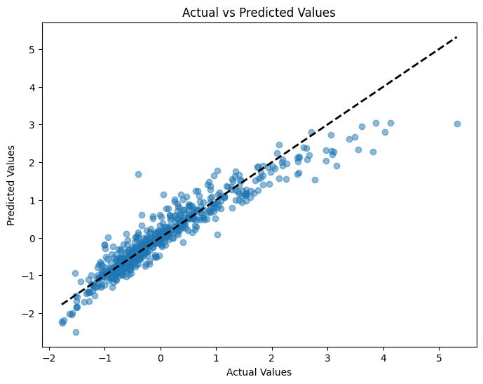
Ridge regression#
Let’s try a Ridge regression now. Note that sklearn uses an \(\alpha\) term, rather than \(\lambda\), like in the text. The two are related. See the footnotes in Chapter 3.
In John Hull’s textbook, this penalty is written using the symbol \lambda , but in sklearn Ridge regression, the equivalent parameter is called \alpha . As noted in the footnote in Chapter 3, Python’s Ridge implementation defines:
\(\text{penalty term} = \alpha \sum_{j=1}^{k} \beta_j^2\)
In contrast, Hull defines the Ridge penalty as:
\(\frac{\lambda}{n} \sum_{j=1}^{k} \beta_j^2\)
To align with Hull’s presentation, we multiply Hull’s \(\lambda\) by the number of observations \(n\) to get the corresponding \(\alpha\) for Python. If our training data has 1800 rows, then:
\(\alpha = \lambda \times 1800\)
The code below tries different values of \(\alpha\), fits a Ridge regression for each, and reports the Mean Squared Error (MSE) on a validation set.
As \(\alpha\) increases, the model applies more shrinkage to the coefficients — pulling them closer to zero. This reduces model complexity, which can help prevent overfitting, but it may also hurt performance if the penalty is too aggressive.
What we’re looking for is a sweet spot — a value of \(\alpha\) large enough to reduce overfitting, but not so large that the model underfits.
# The alpha used by Python's ridge should be the lambda in Hull's book times the number of observations
alphas=[0.01*1800, 0.02*1800, 0.03*1800, 0.04*1800, 0.05*1800, 0.075*1800,0.1*1800,0.2*1800, 0.4*1800]
mses=[]
for alpha in alphas:
    ridge=Ridge(alpha=alpha)
    ridge.fit(X_train,y_train)
    pred=ridge.predict(X_val)
    mses.append(mse(y_val,pred))
    print(mse(y_val,pred))
0.11703284346091337
0.11710797319752984
0.11723952924901117
0.11741457158889508
0.1176238406871146
0.11825709631198014
0.11900057469147927
0.1225464999629295
0.13073599680747128
After running this, you might want to plot the MSEs against \(\alpha\) values to visualize the bias–variance tradeoff. You’re likely to see a U-shaped curve:
Small \(\alpha\) → low bias but high variance (potential overfitting)
Large \(\alpha\) → low variance but high bias (potential underfitting)
We’ll explore this more when we get to model tuning and cross-validation, where we pick the best value of \(\alpha\) automatically.
Let’s plot \(\alpha\) values on the y-axis and MSE on the x-axis.
plt.plot(alphas, mses)
[<matplotlib.lines.Line2D at 0x136c28e00>]
Note that this isn’t exactly what’s in the text. Figure 3.8 has \(\lambda\) on the x-axis and Variance Unexplained on the y-axis. This plot gives the same information, though.
Lasso regression#
Let’s look at a lasso regression. We create the lasso object with a specific alpha hyperparameter. Then, we feed that object the necessary data. We’ll use our training data.
Like Ridge, Lasso regression adds a penalty to the cost function, but instead of squaring the coefficients, it uses their absolute values. This subtle change has a major practical impact.
In sklearn, this is written using alpha instead of \(\lambda\) , and the relationship is:
\(\alpha = \frac{\lambda}{2}\)
You can see this in the footnotes and equations in Hull’s Chapter 3. The division by 2 is how the penalty term is defined under the hood in sklearn. So, to align with Hull’s notation, if you want to use \(\lambda = 0.1\) , you set alpha = 0.05 in your Python code.
After fitting the model, try printing out lasso.coef_ — you’ll likely notice that some coefficients are exactly zero. That’s Lasso’s superpower: it performs automatic feature selection by shrinking some coefficients all the way to zero. This helps create simpler, more interpretable models, especially when many features are irrelevant or highly correlated.
This is particularly useful when you have a lot of predictors, and you want to focus on the most important ones.
# Here we produce results for alpha=0.05 which corresponds to lambda=0.1 in Hull's book
lasso = Lasso(alpha=0.05)
lasso.fit(X_train, y_train)
Lasso(alpha=0.05)In a Jupyter environment, please rerun this cell to show the HTML representation or trust the notebook.
On GitHub, the HTML representation is unable to render, please try loading this page with nbviewer.org.
Parameters
We can output the model using this bit of code. Remember, model specifications are contained in the object created when we fit, or estimate, the model.
# DataFrame with corresponding feature and its respective coefficients
coeffs = pd.DataFrame(
    [
        ['intercept'] + list(X_train.columns),
        list(lasso.intercept_) + list(lasso.coef_)
    ]
).transpose().set_index(0)
coeffs
| 1 | |
|---|---|
| 0 | |
| intercept | -0.0 |
| LotArea | 0.044304 |
| OverallQual | 0.298079 |
| OverallCond | 0.0 |
| YearBuilt | 0.052091 |
| YearRemodAdd | 0.064471 |
| BsmtFinSF1 | 0.115875 |
| BsmtUnfSF | -0.0 |
| TotalBsmtSF | 0.10312 |
| 1stFlrSF | 0.032295 |
| 2ndFlrSF | 0.0 |
| GrLivArea | 0.297065 |
| FullBath | 0.0 |
| HalfBath | 0.0 |
| BedroomAbvGr | -0.0 |
| TotRmsAbvGrd | 0.0 |
| Fireplaces | 0.020404 |
| GarageCars | 0.027512 |
| GarageArea | 0.06641 |
| WoodDeckSF | 0.001029 |
| OpenPorchSF | 0.00215 |
| EnclosedPorch | -0.0 |
| Blmngtn | -0.0 |
| Blueste | -0.0 |
| BrDale | -0.0 |
| BrkSide | 0.0 |
| ClearCr | 0.0 |
| CollgCr | -0.0 |
| Crawfor | 0.0 |
| Edwards | -0.0 |
| Gilbert | 0.0 |
| IDOTRR | -0.0 |
| MeadowV | -0.0 |
| Mitchel | -0.0 |
| Names | -0.0 |
| NoRidge | 0.013209 |
| NPkVill | -0.0 |
| NriddgHt | 0.084299 |
| NWAmes | -0.0 |
| OLDTown | -0.0 |
| SWISU | -0.0 |
| Sawyer | -0.0 |
| SawyerW | -0.0 |
| Somerst | 0.0 |
| StoneBr | 0.016815 |
| Timber | 0.0 |
| Veenker | 0.0 |
| Bsmt Qual | 0.020275 |
Do you see all of the zero values? The lasso model penalizes features that are either unimportant or similar to other variables in the model. Notice how all of the negative weights are gone.
Just like we did with Ridge, let’s try a range of \(\lambda\) values (converted to alpha for Python). This allows us to evaluate how aggressive the Lasso penalty should be. Larger penalties will increase bias but reduce variance, and will eliminate more features.
# We now consider different lambda values. The alphas are half the lambdas
alphas=[0.01/2, 0.02/2, 0.03/2, 0.04/2, 0.05/2, 0.075/2, 0.1/2]
mses=[]
for alpha in alphas:
    lasso=Lasso(alpha=alpha)
    lasso.fit(X_train,y_train)
    pred=lasso.predict(X_val)
    mses.append(mse(y_val,pred))
    print(mse(y_val, pred))
0.11654751909608793
0.11682687945311095
0.11803348353132033
0.12012836764958999
0.12301536903084047
0.13178576395045638
0.1401719458448378
You can now examine: • How the MSE changes as alpha increases • How many coefficients are shrunk to zero for each alpha • Whether there’s a tradeoff between model simplicity and predictive performance
Try printing np.sum(lasso.coef_ == 0) inside the loop if you want to track how many features are removed at each level of regularization.
plt.plot(alphas, mses)
[<matplotlib.lines.Line2D at 0x136cb0350>]
Elastic net#
The text comments that the elastic net model doesn’t really give much of an improvement over lasso. Let’s estimate it here, though.
elastic = ElasticNet(alpha=0.05, l1_ratio=0.8, fit_intercept=True)
elastic.fit(X_train, y_train)
ElasticNet(alpha=0.05, l1_ratio=0.8)In a Jupyter environment, please rerun this cell to show the HTML representation or trust the notebook.
On GitHub, the HTML representation is unable to render, please try loading this page with nbviewer.org.
Parameters
We again create our model object and then fit it with data.
What do the alpha and l1_ratio parameters do? From Claude:
In the scikit-learn implementation of Elastic Net regression (ElasticNet class), the alpha and l1_ratio parameters control the strength and balance between the L1 (Lasso) and L2 (Ridge) regularization penalties, respectively.
alpha (float): This parameter controls the overall strength of the regularization. A higher value of alpha increases the regularization effect, shrinking the coefficients more towards zero. When alpha=0, there is no regularization, and the model becomes a ordinary least squares linear regression.
l1_ratio (float between 0 and 1): This parameter determines the balance between the L1 and L2 penalties in the Elastic Net regularization. Specifically: l1_ratio=1 means the penalty is an L1 penalty (Lasso). l1_ratio=0 means the penalty is an L2 penalty (Ridge). 0 < l1_ratio < 1 means the penalty is a combination of L1 and L2 penalties (Elastic Net).
So, alpha controls the overall regularization strength, while l1_ratio determines how much of that regularization comes from the L1 penalty vs the L2 penalty. In practice, you would tune both alpha and l1_ratio using cross-validation to find the best combination for your specific data. Common values for l1_ratio are 0.5 (balanced Elastic Net), 0.2, or 0.8 depending on whether you want more L2 or L1 regularization respectively.
Let’s look.
# DataFrame with corresponding feature and its respective coefficients
coeffs = pd.DataFrame(
    [
        ['intercept'] + list(X_train.columns),
        list(elastic.intercept_) + list(elastic.coef_)
    ]
).transpose().set_index(0)
coeffs
| 1 | |
|---|---|
| 0 | |
| intercept | -0.0 |
| LotArea | 0.051311 |
| OverallQual | 0.283431 |
| OverallCond | 0.005266 |
| YearBuilt | 0.059446 |
| YearRemodAdd | 0.067086 |
| BsmtFinSF1 | 0.11673 |
| BsmtUnfSF | -0.0 |
| TotalBsmtSF | 0.096558 |
| 1stFlrSF | 0.038404 |
| 2ndFlrSF | 0.0 |
| GrLivArea | 0.29222 |
| FullBath | 0.0 |
| HalfBath | 0.0 |
| BedroomAbvGr | -0.0 |
| TotRmsAbvGrd | 0.0 |
| Fireplaces | 0.025387 |
| GarageCars | 0.030232 |
| GarageArea | 0.066393 |
| WoodDeckSF | 0.005885 |
| OpenPorchSF | 0.011107 |
| EnclosedPorch | -0.0 |
| Blmngtn | -0.0 |
| Blueste | -0.0 |
| BrDale | -0.0 |
| BrkSide | 0.0 |
| ClearCr | 0.0 |
| CollgCr | -0.0 |
| Crawfor | 0.00707 |
| Edwards | 0.0 |
| Gilbert | 0.0 |
| IDOTRR | -0.0 |
| MeadowV | -0.0 |
| Mitchel | -0.0 |
| Names | -0.0 |
| NoRidge | 0.023858 |
| NPkVill | -0.0 |
| NriddgHt | 0.094224 |
| NWAmes | -0.0 |
| OLDTown | -0.0 |
| SWISU | -0.0 |
| Sawyer | -0.0 |
| SawyerW | -0.0 |
| Somerst | 0.0 |
| StoneBr | 0.028336 |
| Timber | 0.0 |
| Veenker | 0.0 |
| Bsmt Qual | 0.025081 |
Watch what happens when I set l1_ratio = 1. I get the lasso model!
elastic = ElasticNet(alpha=0.05, l1_ratio=1, fit_intercept=True)
elastic.fit(X_train, y_train)
ElasticNet(alpha=0.05, l1_ratio=1)In a Jupyter environment, please rerun this cell to show the HTML representation or trust the notebook.
On GitHub, the HTML representation is unable to render, please try loading this page with nbviewer.org.
Parameters
coeffs = pd.DataFrame(
    [
        ['intercept'] + list(X_train.columns),
        list(elastic.intercept_) + list(elastic.coef_)
    ]
).transpose().set_index(0)
coeffs
| 1 | |
|---|---|
| 0 | |
| intercept | -0.0 |
| LotArea | 0.044304 |
| OverallQual | 0.298079 |
| OverallCond | 0.0 |
| YearBuilt | 0.052091 |
| YearRemodAdd | 0.064471 |
| BsmtFinSF1 | 0.115875 |
| BsmtUnfSF | -0.0 |
| TotalBsmtSF | 0.10312 |
| 1stFlrSF | 0.032295 |
| 2ndFlrSF | 0.0 |
| GrLivArea | 0.297065 |
| FullBath | 0.0 |
| HalfBath | 0.0 |
| BedroomAbvGr | -0.0 |
| TotRmsAbvGrd | 0.0 |
| Fireplaces | 0.020404 |
| GarageCars | 0.027512 |
| GarageArea | 0.06641 |
| WoodDeckSF | 0.001029 |
| OpenPorchSF | 0.00215 |
| EnclosedPorch | -0.0 |
| Blmngtn | -0.0 |
| Blueste | -0.0 |
| BrDale | -0.0 |
| BrkSide | 0.0 |
| ClearCr | 0.0 |
| CollgCr | -0.0 |
| Crawfor | 0.0 |
| Edwards | -0.0 |
| Gilbert | 0.0 |
| IDOTRR | -0.0 |
| MeadowV | -0.0 |
| Mitchel | -0.0 |
| Names | -0.0 |
| NoRidge | 0.013209 |
| NPkVill | -0.0 |
| NriddgHt | 0.084299 |
| NWAmes | -0.0 |
| OLDTown | -0.0 |
| SWISU | -0.0 |
| Sawyer | -0.0 |
| SawyerW | -0.0 |
| Somerst | 0.0 |
| StoneBr | 0.016815 |
| Timber | 0.0 |
| Veenker | 0.0 |
| Bsmt Qual | 0.020275 |
Prediction workflow with sklearn#
The Hull textbook often does things “by hand”. For example, he splits the data into training, validation, and test samples by using .iloc and manually slicing the data frame. This is a problem if the data aren’t sorted randomly! He standardizes the variables by using the z-score formula. He searches for optimal hyperparameters by making a graph.
It turns out the sklearn can do a lot of this for us. In fact, if you use tools like Copilot or ChatGPT you’re likely to get code that uses the sklearn workflow. So, we should understand how to use these tools. The fact that ChatGPT wants to use them means that they are extremely common.
This chapter starts off with a discussion of the general workflow, so I’m assuming that you’ve already done your basic data cleaning.
Splitting your data#
Let’s use sklearn and our Zillow data from above to split the data into training and testing samples. From Claude:
train_test_split is a function in the sklearn.model_selection module of the scikit-learn library in Python. It is used to split a dataset into two subsets: a training set and a test set. The training set is used to train a machine learning model, while the test set is used to evaluate its performance on unseen data.
The train_test_split function takes the following arguments:
X: The feature matrix or data frame containing the input variables.
y: The target vector or data frame containing the output variable(s).
test_size (optional): The proportion of the dataset to include in the test split. It should be a float between 0.0 and 1.0. The default value is 0.25, which means 25% of the data will be used for testing.
random_state (optional): An integer value used to seed the random number generator, which ensures reproducibility of the split.
The function returns four objects:
X_train: The training data for the input features.
X_test: The testing data for the input features.
y_train: The training data for the target variable(s).
y_test: The testing data for the target variable(s).
Notice that it doesn’t do the train, validation, and test split from the Hull book. We can do training and validation within the training data set. I’ll take my data frame zillow_data and split into target and features. Remember, logerror was the variable that we were trying to predict.
I added z to all of the names, just so I don’t overwrite my data frames from above.
zillow_sample = zillow_data[['logerror', 'calculatedfinishedsquarefeet', 'lotsizesquarefeet', 'yearbuilt']]

yz = zillow_sample['logerror']
Xz = zillow_sample.drop('logerror', axis=1)

Xz_train, Xz_test, yz_train, yz_test = train_test_split(Xz, yz, test_size=0.2, random_state=42)
That will create four new data frames for you. I would make sure that you’ve cleaned and standardized everything before you split your data.
AI always chooses 42 to seed its random number generated. The answer to everything.
Standardizing your data#
Let’s again use sklearn and our Zillow data from above to standardize our data. From Claude:
In scikit-learn (sklearn), you can standardize your data using the StandardScaler class from the sklearn.preprocessing module. Standardization is a common preprocessing step in machine learning that scales the features to have a mean of 0 and a standard deviation of 1. This can be beneficial for algorithms that are sensitive to feature scales.
scaler = StandardScaler(): Create an instance of the StandardScaler class.
X_scaled = scaler.fit_transform(X): Fit the scaler to the data and transform the data in one step. The fit_transform method first computes the mean and standard deviation of each feature based on the data in X, and then scales the features by subtracting the mean and dividing by the standard deviation.
The fit_transform method returns the scaled feature matrix X_scaled, where each feature now has a mean of 0 and a standard deviation of 1.
I am going to keep a few variables from the Zillow data, including our target logerror.
scaler.fit_transform creates an array. I convert this array back to a data frame and give the data frame the same column names as before.
scaler = StandardScaler()
Xz_train_scaled = scaler.fit_transform(Xz_train)

Xz_train_scaled = pd.DataFrame(Xz_train_scaled, columns=Xz_train.columns)

Xz_train_scaled
| calculatedfinishedsquarefeet | lotsizesquarefeet | yearbuilt | |
|---|---|---|---|
| 0 | -0.788359 | -0.134278 | -0.786796 |
| 1 | -0.721827 | -0.133585 | -0.701616 |
| 2 | 1.191247 | -0.134877 | -0.403486 |
| 3 | -0.152486 | -0.120922 | -0.914566 |
| 4 | -0.875614 | -0.073567 | 0.533494 |
| ... | ... | ... | ... |
| 7251 | -0.224471 | -0.018918 | 1.129754 |
| 7252 | -0.391347 | -0.134278 | -0.488666 |
| 7253 | -0.237560 | -0.138870 | -2.149677 |
| 7254 | -1.267173 | -0.157980 | 0.916804 |
| 7255 | -0.676018 | -0.140959 | -1.894137 |
7256 rows × 3 columns
Notice the steps above. I create the scaler object. It’s defined using StandardScaler() which does the z-score method. I then use .fit_transform() with it. This method combines two tasks. First, it fits the scaling method by taking the mean and standard deviation for all of the features. Then, it transforms my data using the scaler. I save this in a new array, which I then turn back into a data frame.
We need to transform our y, or target variable as well. Again, we’ll pay attention to data types. yz_train is a series, not a data frame. scaler() wants a data frame.
type(yz_train)
pandas.Series
yz_train= pd.DataFrame(yz_train)
yz_train
| logerror | |
|---|---|
| 2919 | 0.0247 |
| 4298 | -0.1120 |
| 5082 | 0.1458 |
| 1643 | -0.0182 |
| 7624 | 0.1178 |
| ... | ... |
| 5734 | 0.0478 |
| 5191 | 0.0611 |
| 5390 | -0.0502 |
| 860 | -0.0060 |
| 7270 | 0.0286 |
7256 rows × 1 columns
yz_train_scaled = scaler.fit_transform(yz_train)

yz_train_scaled = pd.DataFrame(yz_train_scaled, columns=yz_train.columns)

yz_train_scaled
| logerror | |
|---|---|
| 0 | 0.088347 |
| 1 | -0.799853 |
| 2 | 0.875187 |
| 3 | -0.190393 |
| 4 | 0.693259 |
| ... | ... |
| 7251 | 0.238438 |
| 7252 | 0.324854 |
| 7253 | -0.398311 |
| 7254 | -0.111124 |
| 7255 | 0.113687 |
7256 rows × 1 columns
Now, what about the testing data? From Claude:
When scaling your test data using scikit-learn’s scalers (e.g., StandardScaler, MinMaxScaler, etc.), you should use the mean and standard deviation (or the minimum and maximum values for MinMaxScaler) computed from the training data. This is to ensure that the test data is scaled using the same parameters as the training data, which is crucial for preventing data leakage and maintaining consistency between the training and testing data distributions.
Watch my steps here, as they are different from above. I again create my scaler object, calling it scaler. You could create multiple scalers with different names if you wanted to.
I then fit this scaler using my unscaled training data. This is what I did above, except there I used .fit_transform, which fits the scaler and then transforms the data, all in one step. Now, I’m fitting my scaler with one data set and then transforming a different data set.
I then take this fitted scaler that has the means and standard deviations from my training data. I use those to transform my testing data.
scaler = StandardScaler()
scaler.fit(Xz_train)
Xz_test_scaled = scaler.transform(Xz_test)
I follow the same logic for my y target test data.
yz_test= pd.DataFrame(yz_test)
yz_test
| logerror | |
|---|---|
| 447 | 0.0227 |
| 3018 | 0.4337 |
| 8579 | 0.3941 |
| 5509 | -0.0182 |
| 5279 | 0.0030 |
| ... | ... |
| 6658 | 0.2191 |
| 6734 | 0.0188 |
| 7904 | -0.0429 |
| 1244 | -0.0736 |
| 8622 | -0.0502 |
1815 rows × 1 columns
yz_train
| logerror | |
|---|---|
| 2919 | 0.0247 |
| 4298 | -0.1120 |
| 5082 | 0.1458 |
| 1643 | -0.0182 |
| 7624 | 0.1178 |
| ... | ... |
| 5734 | 0.0478 |
| 5191 | 0.0611 |
| 5390 | -0.0502 |
| 860 | -0.0060 |
| 7270 | 0.0286 |
7256 rows × 1 columns
scaler = StandardScaler()
scaler.fit(yz_train)
yz_test_scaled = scaler.transform(yz_test)
Cross-validation and hyperparameters#
Let’s discuss an idea called cross validation. We’ve already see this a bit when we split our data into training and validation samples. From Claude:
Cross-validation is a technique used in machine learning to evaluate the performance of a model and tune its hyperparameters. It helps to estimate how well the model will generalize to unseen data, and it is particularly useful when the available data is limited. The main idea behind cross-validation is to split the dataset into two parts: a training set and a validation set. The model is trained on the training set and evaluated on the validation set. This process is repeated multiple times, with different portions of the data being used for training and validation in each iteration.
There are several types of cross-validation techniques, but the most common is k-fold cross-validation. Here’s how it works:
The dataset is randomly partitioned into k equal-sized subsets or “folds”.
One of the k folds is held out as the validation set, and the remaining k-1 folds are used for training the model. The model is trained on the k-1 folds and evaluated on the held-out validation fold.
This process is repeated k times, with each of the k folds being used as the validation set exactly once.
The performance metric (e.g., accuracy, F1-score, mean squared error) is calculated for each iteration, and the final performance is the average of the k iterations.
Cross-validation has several advantages:
It provides a more reliable and unbiased estimate of the model’s performance compared to a single train-test split.
It helps to prevent overfitting by evaluating the model on data that it has not seen during training.
It allows for effective hyperparameter tuning by selecting the hyperparameters that yield the best average performance across the cross-validation folds.
It makes efficient use of the available data by using every data point for both training and validation at some point.
Cross-validation is widely used in machine learning competitions, research, and real-world applications. It is a crucial technique for evaluating and tuning models, especially when dealing with limited data or when it is important to estimate the model’s generalization performance accurately.
We are going to use some built-in cross-validation tools. This means that we don’t have to manually split our data set.
I’m going to go back the the Hull data and combine the training and validation data sets. I’m going to use all of the observations and have sklearn perform the cross-fold validation for me.
Let me create my new data frames. This is the Hull data, so it’s already cleaned up and standardized.
combined_train = pd.concat([train, val], ignore_index=True)

X_combined_train = combined_train.drop('Sale Price', axis=1)
y_combined_train= combined_train[['Sale Price']]
I will now search for the optimal hyperparameter (i.e. alpha) value for a LASSO model using cross-validation. I am going to take each alpha (e.g. 0.001) and try it five times in my training data. Each time, I will “hold out” 20% of my training data, estimate a model on 80% of the data using that alpha value. I’ll save my R-Square value from that model as a measure of fit. I’ll then do that four more times for that alpha parameter, holding out a different 20% of my training data each time. That will give me five different R-Square values for each alpha. I’ll then take an average of those R-Square values as my estimate for how well that alpha value performs. Remember, a larger R-Square means that the model “fits” the data better - the model is better able to use your features to explain your targets.
This process is repeated for each alpha value.
We are going to use GridSearchCV to do this. From Claude:
GridSearchCV is a class in scikit-learn that helps you perform an exhaustive search over specified parameter values for an estimator (a machine learning model or algorithm). It is used to find the optimal combination of hyperparameters that maximizes the performance of a machine learning model on a given dataset.
And a visual explanation of the process.
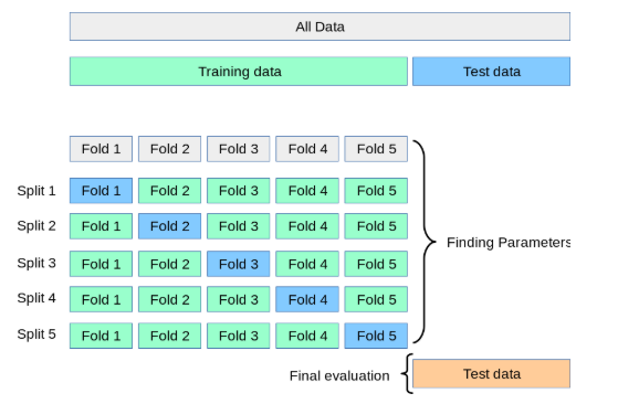
Fig. 91 Holding out different parts of our training data in order to search for optimal hyperparameters. Source:Justintodata.com#
# Tune the LASSO hyperparameter (alpha) using the validation set
param_grid = {'alpha': [0.001, 0.01, 0.02, .05, 0.1]}
grid_search = GridSearchCV(lasso, param_grid, cv=5, scoring='r2')
grid_search.fit(X_combined_train, y_combined_train)

# Extract the R-squared scores for each fold and hyperparameter combination
r2_scores = grid_search.cv_results_['mean_test_score']

# Print the R-squared scores
print(r2_scores)
[0.87838353 0.87833852 0.87472463 0.8567964 0.83113931]
As we already knew, lower alphas give us better results in our training data. We can use this method to select a single set of hyperparameters to then use on our testing data.
Pipelines#
sklearn lets us combine many of these steps together. I’m going to follow along with this example and try something a little fancier. We will use some different model fit statistics to perform cross-validation within our training sample and have the pipeline choose our hyperparameters for us.
pipelines can do much, much more that I show here. Take a look: https://scikit-learn.org/stable/modules/generated/sklearn.pipeline.Pipeline.html
Since I want to use some data that hasn’t been standardized yet, I’ll go back to the Zillow example. I’ll keep some more numerical variables that will be easy to standardize.
I will not include any indicators or other data transformations. If I was doing this for real, I would spend a lot more time doing some feature engineering.
A few things to note:
I’m using
make_pipeline. This is a very common and useful function that let’s you take your features, scale them, define criteria for model selection, etc. You basically transform your data in a series of steps and then ask for the model.I’m asking for the aic criterion. This is a measure of best fit. I will also ask for the bic criterion, another measure of best fit. The smaller the value, the better the model fits the data.
LassoLarsICtells the code to run the lasso model, which we then fit on our training data. This function is going to pick a bunch of alpha values for us, fit the model, and report the requested criterion back to us.
Here’s a description of make_pipeline from Claude GPT:
make_pipelineis a utility function provided by scikit-learn that creates a Pipeline object, which is a sequence of transformers and an estimator. It is a convenient way to chain multiple estimators into a single unit. The make_pipeline function takes any number of estimators as arguments and returns a Pipeline object. The estimators are applied in the order they are passed to the function. The last estimator is always a classifier or regressor, while the other estimators are transformers (preprocessors).Some key features and benefits of using make_pipeline are:
Convenience: It provides a simple and readable way to define a sequence of estimators, making the code more concise and easier to maintain.
Automated Data Flow: The Pipeline object automatically applies the transformers to the input data and passes the transformed data to the final estimator. This avoids the need to manually handle the data flow between estimators.
Consistency: All estimators in the pipeline, except the last one, must be transformers (i.e., have a transform method). This consistency makes it easier to understand and reason about the data flow.
Persistence: The entire pipeline can be persisted to disk using the joblib module, making it easy to reuse the same preprocessing and modeling steps in different environments.
Parallelization: Some transformers in the pipeline can be parallelized using the n_jobs parameter, potentially leading to faster processing times.
Cross-Validation: The entire pipeline can be used in cross-validation loops, ensuring that the same preprocessing steps are applied to both the training and validation data.
Overall, make_pipeline simplifies the process of chaining multiple estimators together and helps to create more readable, maintainable, and efficient code for machine learning workflows.
Here’s my make_pipeline. I am fitting a LASSO model, where I have it use the AIC criteria to pick the “best” hyperparameter. It then fit the model using our new combined training data.
There’s a little bit of data manipulation that make_pipline wants me to do. From Claude:
y_train.values converts the pandas DataFrame y_train to a NumPy array. .ravel() is then applied to the NumPy array, which flattens the array into a 1-dimensional array (required by the LassoLarsIC estimator).
I need to do a little data cleaning on this Zillow data to get it to work in our pipeline.
zillow_sample = zillow_data[['logerror','bathroomcnt', 'bedroomcnt', 'calculatedfinishedsquarefeet', 'fireplacecnt',
       'fullbathcnt', 'garagecarcnt', 'garagetotalsqft','lotsizesquarefeet',
       'poolcnt', 'poolsizesum', 'yearbuilt', 'numberofstories']]
zillow_sample
| logerror | bathroomcnt | bedroomcnt | calculatedfinishedsquarefeet | fireplacecnt | fullbathcnt | garagecarcnt | garagetotalsqft | lotsizesquarefeet | poolcnt | poolsizesum | yearbuilt | numberofstories | |
|---|---|---|---|---|---|---|---|---|---|---|---|---|---|
| 0 | 0.0962 | 3.0 | 2.0 | 1798.0 | NaN | 3.0 | NaN | NaN | 7302.0 | NaN | NaN | 1936.0 | NaN |
| 1 | 0.0020 | 3.0 | 4.0 | 2302.0 | 1.0 | 3.0 | 2.0 | 671.0 | 7258.0 | 1.0 | 500.0 | 1980.0 | 2.0 |
| 2 | -0.0566 | 2.0 | 3.0 | 1236.0 | NaN | 2.0 | NaN | NaN | 5076.0 | NaN | NaN | 1957.0 | NaN |
| 3 | 0.0227 | 2.0 | 2.0 | 1413.0 | NaN | 2.0 | NaN | NaN | 7725.0 | NaN | NaN | 1953.0 | NaN |
| 4 | 0.0237 | 3.5 | 3.0 | 2878.0 | 1.0 | 3.0 | 2.0 | 426.0 | 10963.0 | NaN | NaN | 2003.0 | 1.0 |
| ... | ... | ... | ... | ... | ... | ... | ... | ... | ... | ... | ... | ... | ... |
| 9066 | -0.0305 | 3.0 | 5.0 | 2465.0 | NaN | 3.0 | NaN | NaN | 4999.0 | NaN | NaN | 1931.0 | NaN |
| 9067 | 0.0266 | 3.0 | 3.0 | 1726.0 | NaN | 3.0 | NaN | NaN | 187293.0 | 1.0 | NaN | 1981.0 | NaN |
| 9068 | 0.0090 | 2.0 | 4.0 | 1393.0 | NaN | 2.0 | 2.0 | 451.0 | 6279.0 | NaN | NaN | 1963.0 | 1.0 |
| 9069 | 0.0497 | 2.0 | 3.0 | 1967.0 | NaN | 2.0 | NaN | NaN | 18129.0 | NaN | NaN | 1951.0 | NaN |
| 9070 | -0.0747 | 3.5 | 3.0 | 3268.0 | NaN | 3.0 | 1.0 | 396.0 | 2875.0 | NaN | NaN | 1990.0 | NaN |
9071 rows × 13 columns
For some of these counts, missings are actually zeroes. I can glance at the data and see, however, that this isn’t true for all observations. For example we have a poolcnt = 1, but poolsizesum = 0. I’ll go ahead and just fill in the missings for the purpose of this exercise. But, not great!
# Set missing observations to zero
zillow_sample = zillow_sample.fillna(0)

zillow_sample
| logerror | bathroomcnt | bedroomcnt | calculatedfinishedsquarefeet | fireplacecnt | fullbathcnt | garagecarcnt | garagetotalsqft | lotsizesquarefeet | poolcnt | poolsizesum | yearbuilt | numberofstories | |
|---|---|---|---|---|---|---|---|---|---|---|---|---|---|
| 0 | 0.0962 | 3.0 | 2.0 | 1798.0 | 0.0 | 3.0 | 0.0 | 0.0 | 7302.0 | 0.0 | 0.0 | 1936.0 | 0.0 |
| 1 | 0.0020 | 3.0 | 4.0 | 2302.0 | 1.0 | 3.0 | 2.0 | 671.0 | 7258.0 | 1.0 | 500.0 | 1980.0 | 2.0 |
| 2 | -0.0566 | 2.0 | 3.0 | 1236.0 | 0.0 | 2.0 | 0.0 | 0.0 | 5076.0 | 0.0 | 0.0 | 1957.0 | 0.0 |
| 3 | 0.0227 | 2.0 | 2.0 | 1413.0 | 0.0 | 2.0 | 0.0 | 0.0 | 7725.0 | 0.0 | 0.0 | 1953.0 | 0.0 |
| 4 | 0.0237 | 3.5 | 3.0 | 2878.0 | 1.0 | 3.0 | 2.0 | 426.0 | 10963.0 | 0.0 | 0.0 | 2003.0 | 1.0 |
| ... | ... | ... | ... | ... | ... | ... | ... | ... | ... | ... | ... | ... | ... |
| 9066 | -0.0305 | 3.0 | 5.0 | 2465.0 | 0.0 | 3.0 | 0.0 | 0.0 | 4999.0 | 0.0 | 0.0 | 1931.0 | 0.0 |
| 9067 | 0.0266 | 3.0 | 3.0 | 1726.0 | 0.0 | 3.0 | 0.0 | 0.0 | 187293.0 | 1.0 | 0.0 | 1981.0 | 0.0 |
| 9068 | 0.0090 | 2.0 | 4.0 | 1393.0 | 0.0 | 2.0 | 2.0 | 451.0 | 6279.0 | 0.0 | 0.0 | 1963.0 | 1.0 |
| 9069 | 0.0497 | 2.0 | 3.0 | 1967.0 | 0.0 | 2.0 | 0.0 | 0.0 | 18129.0 | 0.0 | 0.0 | 1951.0 | 0.0 |
| 9070 | -0.0747 | 3.5 | 3.0 | 3268.0 | 0.0 | 3.0 | 1.0 | 396.0 | 2875.0 | 0.0 | 0.0 | 1990.0 | 0.0 |
9071 rows × 13 columns
yz = zillow_sample.loc[:, 'logerror']
Xz = zillow_sample.drop('logerror', axis=1)

Xz_train, Xz_test, yz_train, yz_test = train_test_split(Xz, yz, test_size=0.2, random_state=42)
Xz_train
| bathroomcnt | bedroomcnt | calculatedfinishedsquarefeet | fireplacecnt | fullbathcnt | garagecarcnt | garagetotalsqft | lotsizesquarefeet | poolcnt | poolsizesum | yearbuilt | numberofstories | |
|---|---|---|---|---|---|---|---|---|---|---|---|---|
| 2919 | 1.0 | 2.0 | 1041.0 | 0.0 | 1.0 | 1.0 | 360.0 | 6120.0 | 0.0 | 0.0 | 1950.0 | 1.0 |
| 4298 | 1.0 | 3.0 | 1102.0 | 0.0 | 1.0 | 0.0 | 0.0 | 6259.0 | 1.0 | 0.0 | 1952.0 | 0.0 |
| 5082 | 3.5 | 6.0 | 2856.0 | 0.0 | 3.0 | 1.0 | 360.0 | 6000.0 | 0.0 | 0.0 | 1959.0 | 1.0 |
| 1643 | 3.0 | 4.0 | 1624.0 | 0.0 | 3.0 | 0.0 | 0.0 | 8799.0 | 0.0 | 0.0 | 1947.0 | 0.0 |
| 7624 | 2.0 | 2.0 | 961.0 | 0.0 | 2.0 | 0.0 | 0.0 | 18297.0 | 0.0 | 0.0 | 1981.0 | 0.0 |
| ... | ... | ... | ... | ... | ... | ... | ... | ... | ... | ... | ... | ... |
| 5734 | 3.0 | 2.0 | 1558.0 | 0.0 | 3.0 | 0.0 | 0.0 | 29258.0 | 1.0 | 0.0 | 1995.0 | 0.0 |
| 5191 | 2.0 | 4.0 | 1405.0 | 0.0 | 2.0 | 2.0 | 441.0 | 6120.0 | 0.0 | 0.0 | 1957.0 | 1.0 |
| 5390 | 2.0 | 3.0 | 1546.0 | 0.0 | 2.0 | 0.0 | 0.0 | 5199.0 | 0.0 | 0.0 | 1918.0 | 0.0 |
| 860 | 1.0 | 1.0 | 602.0 | 0.0 | 1.0 | 1.0 | 0.0 | 1366.0 | 0.0 | 0.0 | 1990.0 | 0.0 |
| 7270 | 1.0 | 2.0 | 1144.0 | 0.0 | 1.0 | 0.0 | 0.0 | 4780.0 | 0.0 | 0.0 | 1924.0 | 0.0 |
7256 rows × 12 columns
Xz_test
| bathroomcnt | bedroomcnt | calculatedfinishedsquarefeet | fireplacecnt | fullbathcnt | garagecarcnt | garagetotalsqft | lotsizesquarefeet | poolcnt | poolsizesum | yearbuilt | numberofstories | |
|---|---|---|---|---|---|---|---|---|---|---|---|---|
| 447 | 2.0 | 2.0 | 1671.0 | 1.0 | 2.0 | 1.0 | 389.0 | 1750.0 | 0.0 | 0.0 | 1981.0 | 3.0 |
| 3018 | 1.0 | 3.0 | 859.0 | 0.0 | 1.0 | 0.0 | 0.0 | 3456.0 | 0.0 | 0.0 | 1940.0 | 0.0 |
| 8579 | 2.0 | 4.0 | 1840.0 | 0.0 | 2.0 | 0.0 | 0.0 | 7173.0 | 0.0 | 0.0 | 1965.0 | 0.0 |
| 5509 | 2.0 | 4.0 | 1200.0 | 0.0 | 2.0 | 0.0 | 0.0 | 7740.0 | 0.0 | 0.0 | 1955.0 | 0.0 |
| 5279 | 2.5 | 3.0 | 1604.0 | 0.0 | 2.0 | 2.0 | 0.0 | 0.0 | 0.0 | 0.0 | 1989.0 | 0.0 |
| ... | ... | ... | ... | ... | ... | ... | ... | ... | ... | ... | ... | ... |
| 6658 | 2.0 | 2.0 | 947.0 | 0.0 | 2.0 | 0.0 | 0.0 | 72341.0 | 0.0 | 0.0 | 1974.0 | 0.0 |
| 6734 | 2.0 | 3.0 | 1974.0 | 0.0 | 2.0 | 0.0 | 0.0 | 6304.0 | 0.0 | 0.0 | 1964.0 | 0.0 |
| 7904 | 3.0 | 2.0 | 1888.0 | 0.0 | 3.0 | 0.0 | 0.0 | 122753.0 | 1.0 | 0.0 | 1972.0 | 0.0 |
| 1244 | 1.0 | 1.0 | 600.0 | 0.0 | 1.0 | 0.0 | 0.0 | 46486.0 | 1.0 | 0.0 | 2004.0 | 0.0 |
| 8622 | 3.5 | 4.0 | 3327.0 | 2.0 | 3.0 | 3.0 | 732.0 | 26332.0 | 1.0 | 648.0 | 2001.0 | 1.0 |
1815 rows × 12 columns
yz_train
2919    0.0247
4298   -0.1120
5082    0.1458
1643   -0.0182
7624    0.1178
         ...
5734    0.0478
5191    0.0611
5390   -0.0502
860    -0.0060
7270    0.0286
Name: logerror, Length: 7256, dtype: float64
yz_test
447     0.0227
3018    0.4337
8579    0.3941
5509   -0.0182
5279    0.0030
         ...
6658    0.2191
6734    0.0188
7904   -0.0429
1244   -0.0736
8622   -0.0502
Name: logerror, Length: 1815, dtype: float64
Time to make the pipeline. This is going to use the standard scaler on my training data and run a Lasso model, here the hyperparameter is selected using the AIC criteria.
Again, note how the X features set is are data frames, while the y target set are series.
lasso_lars_ic = make_pipeline(StandardScaler(), LassoLarsIC(criterion="aic")).fit(Xz_train, yz_train.values.ravel())
results = pd.DataFrame(
    {
        "alphas": lasso_lars_ic[-1].alphas_,
        "AIC criterion": lasso_lars_ic[-1].criterion_,
    }
).set_index("alphas")
alpha_aic = lasso_lars_ic[-1].alpha_
Same thing as above, but now using the BIC selection criteria.
lasso_lars_ic.set_params(lassolarsic__criterion="bic").fit(Xz_train, yz_train.values.ravel())
results["BIC criterion"] = lasso_lars_ic[-1].criterion_
alpha_bic = lasso_lars_ic[-1].alpha_
You can see below that small values of alpha give us the best model fit, no matter the criteria used. This confirms what we saw graphically above.
def highlight_min(x):
    x_min = x.min()
    return ["font-weight: bold" if v == x_min else "" for v in x]

results.style.apply(highlight_min)
| AIC criterion | BIC criterion | |
|---|---|---|
| alphas | ||
| 0.008193 | -6566.197538 | -6566.197538 |
| 0.006502 | -6571.833764 | -6564.944180 |
| 0.006250 | -6570.829907 | -6557.050739 |
| 0.006217 | -6568.983921 | -6548.315169 |
| 0.005552 | -6572.082467 | -6551.413715 |
| 0.004159 | -6577.437720 | -6556.768968 |
| 0.004015 | -6576.114858 | -6548.556522 |
| 0.002618 | -6581.223880 | -6546.775960 |
| 0.002365 | -6580.648359 | -6539.310855 |
| 0.000653 | -6587.044949 | -6538.817861 |
| 0.000577 | -6585.219803 | -6530.103131 |
| 0.000412 | -6583.581262 | -6521.575006 |
| 0.000239 | -6582.063000 | -6513.167160 |
| 0.000168 | -6580.302964 | -6504.517540 |
| 0.000000 | -6580.414299 | -6497.739291 |
This table highlights the optimal alpha hyperparameter based on two different selection criteria.
Let’s make a plot. We’ll use matplotlib and the ax method.
ax = results.plot()
ax.vlines(
    alpha_aic,
    results["AIC criterion"].min(),
    results["AIC criterion"].max(),
    label="alpha: AIC estimate",
    linestyles="--",
    color="tab:blue",
)
ax.vlines(
    alpha_bic,
    results["BIC criterion"].min(),
    results["BIC criterion"].max(),
    label="alpha: BIC estimate",
    linestyle="--",
    color="tab:orange",
)
ax.set_xlabel(r"$\alpha$")
ax.set_ylabel("criterion")
ax.set_xscale("log")
ax.legend()
_ = ax.set_title(
    f"Information-criterion for model selection"
)
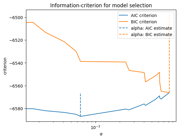
This doesn’t look as continuous as it will in practice. The lines are jumping around quite a bit. The reason: We actually don’t have that many features in this Zillow data set that I’m using. Our machine learning tools will work, but are probably unnecessary. Just run a regression!
Let’s create a new pipeline using cross-validation, rather than using the AIC or BIC criteria. What’s the difference? From Claude:
LassoCV uses cross-validation to find the optimal alpha value that minimizes a chosen scoring metric, making it more robust but computationally expensive. LassoLarsIC(criterion=”aic”) uses the Akaike Information Criterion (AIC) to find the optimal alpha value, providing a faster but potentially less accurate estimate than cross-validation.
modelcv = make_pipeline(LassoCV(cv=20)).fit(Xz_train, yz_train)
Again, modelcv is a pipeline. A pipeline is an object. This object contains our lasso model fit. We’ll pull this out below and define it as lasso.
modelcv
Pipeline(steps=[('lassocv', LassoCV(cv=20))])In a Jupyter environment, please rerun this cell to show the HTML representation or trust the notebook. On GitHub, the HTML representation is unable to render, please try loading this page with nbviewer.org.
Parameters
Parameters
lasso = modelcv[-1]
lasso
LassoCV(cv=20)In a Jupyter environment, please rerun this cell to show the HTML representation or trust the notebook.
On GitHub, the HTML representation is unable to render, please try loading this page with nbviewer.org.
Parameters
OK, what did we do here? Let’s have Claude tell us:
In scikit-learn, LassoCV(cv=20) refers to the Lasso regression model with cross-validation for tuning the regularization parameter (alpha). Here’s what the components mean:
LassoCV: This is the class name for the Lasso regression model with built-in cross-validation for automatically tuning the regularization strength parameter (alpha).
cv=20: This is a parameter that specifies the number of folds for cross-validation. In this case, it means that the cross-validation process will be repeated 20 times, each time using a different 1/20th of the data as the validation set and the remaining 19/20ths as the training set.
The LassoCV class performs the following steps:
It splits the data into cv (20 in this case) folds or subsets.
For each fold:
2a. It holds out that fold as the validation set.
2b. It trains the Lasso regression model on the remaining cv-1 folds, using a range of different alpha values.
2c. It evaluates the performance of the model on the held-out validation fold for each alpha value.
After all folds have been processed, it selects the alpha value that gives the best average performance across all folds.
Finally, it retrains the Lasso regression model on the entire dataset using the optimal alpha value found through cross-validation.
By using cross-validation, LassoCV can automatically find the optimal value of the regularization parameter (alpha) that balances the trade-off between model complexity and goodness of fit. This helps to prevent overfitting and improve the model’s generalization performance. The choice of cv = 20 is a common practice, as it provides a good balance between computational cost and reliable estimation of the model’s performance. However, the optimal value of cv can depend on the size of the dataset and the complexity of the problem.
I can print out the parameters contained in my LASSO model. This will tell you the details of how things were estimated.
lasso.get_params()
{'alphas': 'warn',
 'copy_X': True,
 'cv': 20,
 'eps': 0.001,
 'fit_intercept': True,
 'max_iter': 1000,
 'n_alphas': 'deprecated',
 'n_jobs': None,
 'positive': False,
 'precompute': 'auto',
 'random_state': None,
 'selection': 'cyclic',
 'tol': 0.0001,
 'verbose': False}
I can also pull out the hyperparameter that was eventually chosen using cross-validation.
lasso.alpha_
0.9233932158250625
That’s a large hyperparameter. Lots of features were dropped. Let’s look.
I’ll make a table that has the coefficients from the final model estimated using my training data. Square feet of house and lot are all that are selected. The LASSO model drops every other feature.
feature_names = list(Xz_train.columns)
coefficients = lasso.coef_

# Create a DataFrame with feature names and coefficients
coef_df = pd.DataFrame({'Feature': feature_names, 'Coefficient': coefficients})

# Sort the DataFrame by the absolute value of coefficients in descending order
coef_df = coef_df.reindex(coef_df['Coefficient'].abs().sort_values(ascending=False).index)

coef_df
| Feature | Coefficient | |
|---|---|---|
| 2 | calculatedfinishedsquarefeet | 7.260294e-06 |
| 7 | lotsizesquarefeet | 1.356992e-08 |
| 0 | bathroomcnt | 0.000000e+00 |
| 1 | bedroomcnt | 0.000000e+00 |
| 3 | fireplacecnt | 0.000000e+00 |
| 4 | fullbathcnt | 0.000000e+00 |
| 5 | garagecarcnt | 0.000000e+00 |
| 6 | garagetotalsqft | 0.000000e+00 |
| 8 | poolcnt | 0.000000e+00 |
| 9 | poolsizesum | -0.000000e+00 |
| 10 | yearbuilt | 0.000000e+00 |
| 11 | numberofstories | 0.000000e+00 |
And, we can print the R2 for the final model from the training data.
score = modelcv.score(Xz_train, yz_train)
print(f"Test score: {score}")
Test score: 0.002722552194950545
Well, that’s terrible! But, again, we’re trying to predict pricing errors with only a subset of the features. Predicting actual housing prices is much easier.
I’m going to print my mse values in order to find some reasonable min and max values for the graph below. Remember, our target is the log of the pricing error. This isn’t a dollar amount for the house.
See how I’m just pulling things out of my lasso object? It contains all of this information about our estimated model.
lasso.mse_path_
array([[0.01496657, 0.0125596 , 0.01200737, ..., 0.02217262, 0.01876269,
        0.04859113],
       [0.01496652, 0.01255985, 0.01200748, ..., 0.02217262, 0.01876246,
        0.04859252],
       [0.01496649, 0.01256036, 0.01200758, ..., 0.02217262, 0.01876225,
        0.04859384],
       ...,
       [0.01484608, 0.01278774, 0.01219113, ..., 0.02204339, 0.01876977,
        0.04869556],
       [0.01484857, 0.01278637, 0.01219214, ..., 0.02204383, 0.0187697 ,
        0.04870231],
       [0.01485083, 0.01278511, 0.0121931 , ..., 0.02204417, 0.01876976,
        0.04870873]])
ymin, ymax = 0, 0.2

plt.semilogx(lasso.alphas_, lasso.mse_path_, linestyle=":")
plt.plot(
    lasso.alphas_,
    lasso.mse_path_.mean(axis=-1),
    color="black",
    label="Average across the folds",
    linewidth=2,
)
plt.axvline(lasso.alpha_, linestyle="--", color="black", label="alpha: CV estimate")

plt.ylim(ymin, ymax)
plt.xlabel(r"$\alpha$")
plt.ylabel("Mean square error")
plt.legend()
_ = plt.title(
    f"Mean square error on each fold: coordinate descent"
)
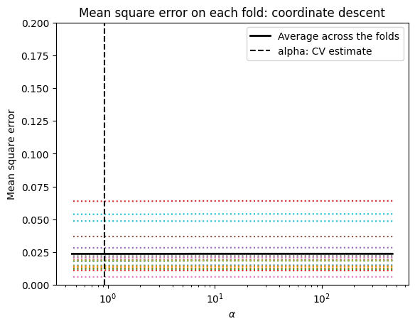
Finally, I’m going to use my fitted model from my training data on my testing data. I’ll print the R2 value as a measure of how well we predict
# Evaluate the model on the test data
score = modelcv.score(Xz_test, yz_test)
print(f"Test score: {score}")
Test score: 0.0028149345560726236
Still bad! I guess if you squint, it’s a little better than what we did in the training data.
Hyperparameters and model overfit#
Again, what’s the point of all of this? We’re trying to find our model hyperparameters that we can then take to data outside of our training set. We are trying to avoid overfitting. This is a problem in machine learning and, especially, in financial applications. It is easy to look at past financial data and fit a model that will predict returns in sample, in the data we are using. But, will this work on new data? If you overfit your model, you risk making precisely incorrect predictions.
The figure below shows this problem clearly. As model complexity increases, training accuracy skyrockets – the model is memorizing the data. But test accuracy (on data the model has never seen) flatlines or even drops. The gap between the two curves is the overfitting.
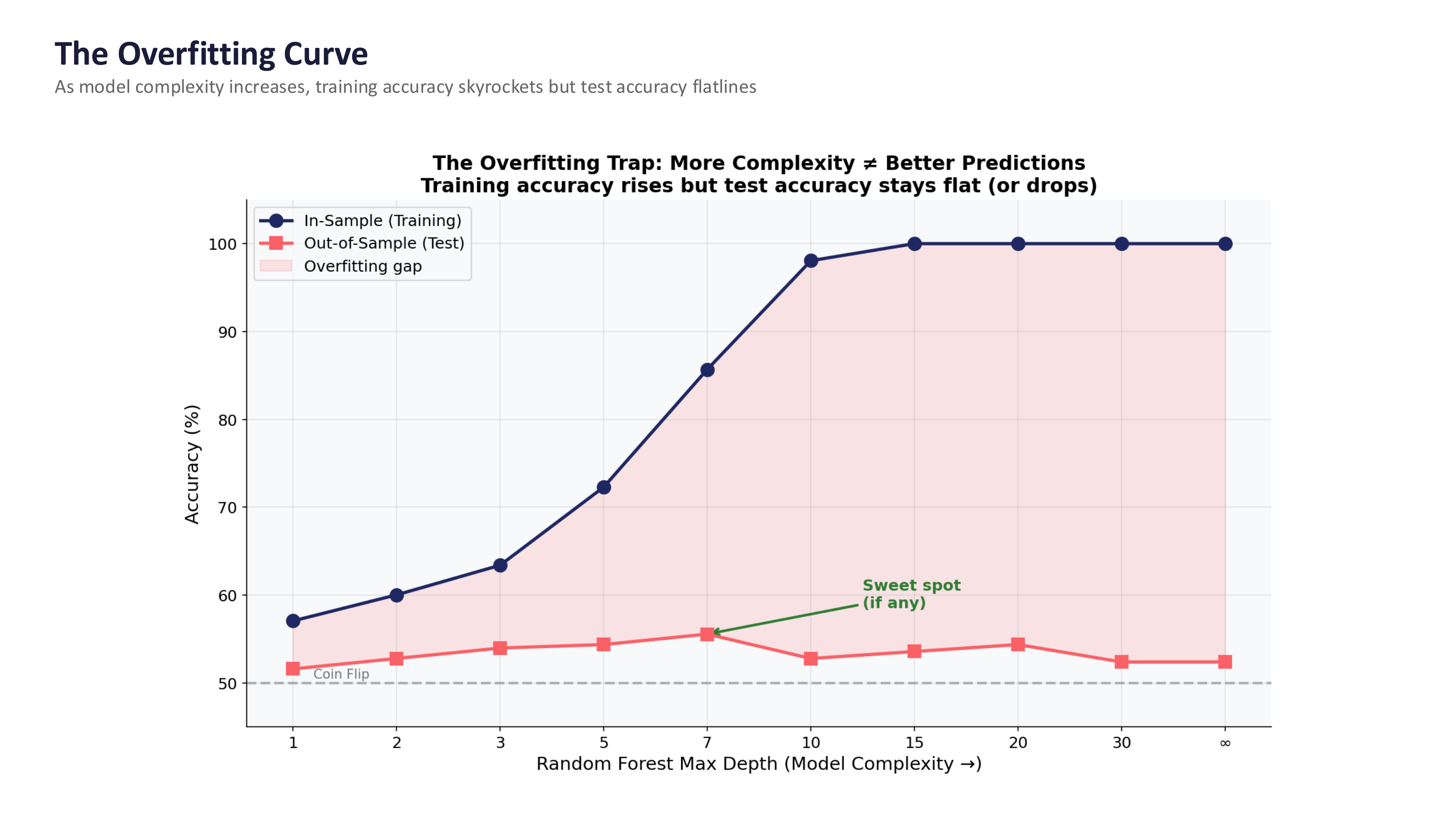
Fig. 92 The overfitting trap: more complexity does not mean better predictions. Training accuracy rises, but test accuracy stays flat. The “sweet spot” (if any) is where test accuracy peaks before declining. Source: Professor Jonathan Hersh, BUS 696: Generative AI in Finance, Chapman University, Spring 2026.#
Warning
The in-sample vs. out-of-sample trap. This is the single most important concept when applying machine learning to finance. Getting 70% accuracy in your training data means almost nothing – the model may have simply memorized noise. The real test is predicting data the model has never seen, and this is where most financial ML models fail. Financial data has a very low signal-to-noise ratio, patterns are non-stationary (what worked last year may not work this year), and if others discover the same pattern, it gets arbitraged away.
Here’s a nice explanation on what is going on. This is all part of a much larger discussion on model selection
Some worked examples#
We are just scratching the surface on machine learning in this course. Here are some complete examples that all use housing price data. Some things to pay attention to:
How are the data organized? How is it split into training and test data?
How is the data quality checked? How are missing values handled? How about outliers?
What feature engineering steps are used? Are logs taken? Are there categorical variables in the regressions? Are the variables scaled?
What visualizations are used to look at the data before modeling? Why are they used?
What models are used? How are they compared?
From Regression to Prediction: Can ML Beat the Market?#
We have now covered OLS regression, Lasso, Ridge, and Elastic Net. We have learned about train/test splits, cross-validation, and hyperparameter tuning. The natural next question: can we use these tools to predict stock returns?
The short answer is humbling. Let’s walk through what actually happens when you take these models to financial markets.
The model horse race#
A common exercise in machine learning is the model horse race – train several models on the same data and compare their performance. When researchers do this with stock market data (e.g., predicting whether the S&P 500 goes up or down), a striking pattern emerges.
Fig. 93 The model horse race: predicting S&P 500 direction. Complex models look great in-sample but collapse out-of-sample. Source: Professor Jonathan Hersh, BUS 696: Generative AI in Finance, Chapman University, Spring 2026.#
Look at the pattern in the figure. In-sample (training data), more complex models do better – Lasso beats logistic regression, and tree-based models beat Lasso. XGBoost can hit 97% accuracy in the training data! But out-of-sample (test data), they all collapse to roughly 50% – no better than a coin flip.
The more complex the model, the larger the gap between training and test accuracy. This gap is the overfitting. XGBoost memorized the training data perfectly, but learned nothing that generalizes to new data.
Important
This is the most important empirical result in financial ML: model complexity alone does not solve the problem when the signal is weak. Financial returns have an extremely low signal-to-noise ratio. No amount of model sophistication can extract a signal that isn’t there.
What ~52% accuracy actually looks like#
Even the best academic models for predicting market direction tend to land around 51-53% accuracy. That sounds close to 50%, but is it meaningfully different? Let’s look at what this means in practice.
Fig. 94 What ~52% accuracy actually looks like compared to a coin flip. The confusion matrices are nearly identical. Source: Professor Jonathan Hersh, BUS 696: Generative AI in Finance, Chapman University, Spring 2026.#
The figure compares an ML model at 52% accuracy to a random coin flip at ~47%. The confusion matrices look almost identical. The bar chart on the right makes it even clearer – the ML model gets just a handful of extra correct predictions compared to pure randomness.
This is a sobering result. After all of the modeling effort – feature engineering, cross-validation, hyperparameter tuning – you end up barely distinguishable from a coin flip. But here is the key insight: in finance, even a tiny edge can be enormously valuable if you know how to exploit it. The question is not just can you predict? but what do you do with that prediction?
What the smart money actually does#
If model complexity alone doesn’t work, how does anyone make money with ML in finance? The answer is that successful quantitative firms approach the problem very differently from a standard Kaggle competition.
Fig. 95 How quantitative firms actually use ML in practice. Source: Professor Jonathan Hersh, BUS 696: Generative AI in Finance, Chapman University, Spring 2026.#
Here are the key lessons:
Better features, not better models. The alpha comes from unique data, not fancier algorithms. A Lasso on satellite parking lot data beats XGBoost on price history. This is why hedge funds spend millions on alternative data.
Predict something easier. Volatility is far more predictable than returns. Relative rankings (cross-sectional: “which stocks outperform others?”) are easier than absolute predictions (“will AAPL go up?”). Longer horizons (weekly, monthly) have better signal-to-noise than daily.
Ensemble many weak signals. One model at 51% accuracy is useless after transaction costs. But combine 100 weakly correlated 51% signals, and you get something real. This is the business model behind firms like Numerai, which crowdsources signals from thousands of data scientists.
Build in transaction costs. A signal that says “trade every day” but the bid-ask spread eats your profit is worthless. The best shops optimize net-of-cost returns.
Walk-forward validation. Don’t just split train/test once. Retrain the model every month on a rolling window. Markets are non-stationary: a model trained on 2020 data may be useless in 2025.
Note
ML works in finance, but not the way you’d naively expect. It’s about finding unique data, asking the right question, and managing risk – not about finding the most complex model.
Position sizing > prediction accuracy#
Perhaps the most surprising lesson from quantitative finance is this: how much you bet matters more than how often you’re right. This is where the Kelly Criterion comes in.
Fig. 96 Position sizing with a 52% win rate. Same edge, very different outcomes depending on bet size. The Kelly Criterion identifies the optimal bet size. Source: Professor Jonathan Hersh, BUS 696: Generative AI in Finance, Chapman University, Spring 2026.#
The figure tells a powerful story. Both lines in the left panel start with the same 52% edge. But the Kelly-optimal strategy (betting ~4% of capital) grows steadily, while betting 20% or 50% of capital leads to ruin. The right panel shows the Kelly Curve – there is an optimal bet size, and betting too much is catastrophic.
The takeaway: the prediction model is only half the system. Portfolio construction – how you size positions, manage risk, and control for transaction costs – matters just as much, if not more. A mediocre model with excellent risk management will beat a great model with poor risk management every time.
Tip
This is why finance programs teach portfolio theory alongside data science. The prediction is just the input. What you do with that prediction – how you size the trade, when you exit, how you hedge – determines whether you make or lose money.