
Merging and reshaping data#
We are going to cover a few topics in this brief section. First, we want to learn about merging or joining data sets. Think of this like xlookup in Excel, or, more generally, SQL queries. In fact, you can do SQL in Python, if you’re familiar with it. We will also see concatenating, or stacking data. We will see how to reshape our data. We’ll see wide and long data. We’ll end with using multi-level indices to shape our data.
I’ll work through a few common examples below using stock data.
Here are some visualizations for what these different functions do.
Tip
AI is your reshaping guide. Figuring out whether you need melt, pivot, stack, unstack, or merge can be confusing. Just describe what you have and what you want: “I have a DataFrame with columns date, aapl_price, msft_price. I want a DataFrame with columns date, ticker, price.” Claude will tell you exactly which function to use and write the code.
# Set-up

import numpy as np
import pandas as pd

import matplotlib as mpl

import matplotlib.pyplot as plt

# Load AAPL and XOM stock data from GitHub
aapl = pd.read_csv('https://raw.githubusercontent.com/aaiken1/fin-data-analysis-python/main/data/aapl.csv')
xom = pd.read_csv('https://raw.githubusercontent.com/aaiken1/fin-data-analysis-python/main/data/xom.csv')

# These CSV files contain historical stock prices and returns

aapl = aapl.set_index('date')
xom = xom.set_index('date')

aapl.info()
<class 'pandas.core.frame.DataFrame'>
Index: 757 entries, 20190102 to 20211231
Data columns (total 14 columns):
 #   Column   Non-Null Count  Dtype
---  ------   --------------  -----
 0   PERMNO   757 non-null    int64
 1   TICKER   757 non-null    object
 2   CUSIP    757 non-null    int64
 3   DISTCD   13 non-null     float64
 4   DIVAMT   13 non-null     float64
 5   FACPR    13 non-null     float64
 6   FACSHR   13 non-null     float64
 7   PRC      757 non-null    float64
 8   VOL      757 non-null    int64
 9   RET      757 non-null    float64
 10  SHROUT   757 non-null    int64
 11  CFACPR   757 non-null    int64
 12  CFACSHR  757 non-null    int64
 13  sprtrn   757 non-null    float64
dtypes: float64(7), int64(6), object(1)
memory usage: 88.7+ KB
Our usual set-up is above. Notice that I’m setting the index of each DataFrame using .set_index(), instead of doing it inside of the .read_csv(). Either way works.
When we set date as our index using .set_index(), it becomes the primary identifier for each row. This means it no longer appears as a regular column, but instead is used to label each row for easier lookups and time-series operations.
xom.info()
<class 'pandas.core.frame.DataFrame'>
Index: 756 entries, 20190102 to 20211230
Data columns (total 14 columns):
 #   Column   Non-Null Count  Dtype
---  ------   --------------  -----
 0   PERMNO   756 non-null    int64
 1   TICKER   756 non-null    object
 2   CUSIP    756 non-null    object
 3   DISTCD   12 non-null     float64
 4   DIVAMT   12 non-null     float64
 5   FACPR    12 non-null     float64
 6   FACSHR   12 non-null     float64
 7   PRC      756 non-null    float64
 8   VOL      756 non-null    int64
 9   RET      756 non-null    float64
 10  SHROUT   756 non-null    int64
 11  CFACPR   756 non-null    int64
 12  CFACSHR  756 non-null    int64
 13  sprtrn   756 non-null    float64
dtypes: float64(7), int64(5), object(2)
memory usage: 88.6+ KB
To confirm that date is now the index, we can use .info().
This command prints:
The total number of rows and columns.
Data types of each column.
Whether an index is set (look at the first line, where it should mention “Index: Int64Index” instead of a column name).
xom.index
Index([20190102, 20190103, 20190104, 20190107, 20190108, 20190109, 20190110,
       20190111, 20190114, 20190115,
       ...
       20211216, 20211217, 20211220, 20211221, 20211222, 20211223, 20211227,
       20211228, 20211229, 20211230],
      dtype='int64', name='date', length=756)
Concatenating data sets#
Appending, or concatenation, or stacking data. This is when you simply put one data set on top of another. However, you need to be careful! Do the data sets share the same variables? How are index values handled?
You can use .concat() from pandas. Notice that our two datasets don’t have exactly the same number of rows. Older code might use .append() from pandas.
pd.concat((aapl, xom), sort=False)
| PERMNO | TICKER | CUSIP | DISTCD | DIVAMT | FACPR | FACSHR | PRC | VOL | RET | SHROUT | CFACPR | CFACSHR | sprtrn | |
|---|---|---|---|---|---|---|---|---|---|---|---|---|---|---|
| date | ||||||||||||||
| 20190102 | 14593 | AAPL | 3783310 | NaN | NaN | NaN | NaN | 157.92000 | 37066356 | 0.001141 | 4729803 | 4 | 4 | 0.001269 |
| 20190103 | 14593 | AAPL | 3783310 | NaN | NaN | NaN | NaN | 142.19000 | 91373695 | -0.099607 | 4729803 | 4 | 4 | -0.024757 |
| 20190104 | 14593 | AAPL | 3783310 | NaN | NaN | NaN | NaN | 148.25999 | 58603001 | 0.042689 | 4729803 | 4 | 4 | 0.034336 |
| 20190107 | 14593 | AAPL | 3783310 | NaN | NaN | NaN | NaN | 147.92999 | 54770364 | -0.002226 | 4729803 | 4 | 4 | 0.007010 |
| 20190108 | 14593 | AAPL | 3783310 | NaN | NaN | NaN | NaN | 150.75000 | 41026062 | 0.019063 | 4729803 | 4 | 4 | 0.009695 |
| ... | ... | ... | ... | ... | ... | ... | ... | ... | ... | ... | ... | ... | ... | ... |
| 20211223 | 11850 | XOM | 30231G10 | NaN | NaN | NaN | NaN | 61.02000 | 13543291 | 0.000492 | 4233567 | 1 | 1 | 0.006224 |
| 20211227 | 11850 | XOM | 30231G10 | NaN | NaN | NaN | NaN | 61.89000 | 12596340 | 0.014258 | 4233567 | 1 | 1 | 0.013839 |
| 20211228 | 11850 | XOM | 30231G10 | NaN | NaN | NaN | NaN | 61.69000 | 12786873 | -0.003232 | 4233567 | 1 | 1 | -0.001010 |
| 20211229 | 11850 | XOM | 30231G10 | NaN | NaN | NaN | NaN | 61.15000 | 12733601 | -0.008753 | 4233567 | 1 | 1 | 0.001402 |
| 20211230 | 11850 | XOM | 30231G10 | NaN | NaN | NaN | NaN | 60.79000 | 11940294 | -0.005887 | 4233567 | 1 | 1 | -0.002990 |
1513 rows × 14 columns
See how there are 1513 rows, but the index for XOM only goes to 755? We didn’t ignore the index, so the original index comes over. The first observation of both DataFrames starts at 0. There are 756 AAPL observations and 755 XOM.
Let’s ignore the index now.
pd.concat((aapl, xom), ignore_index=True, sort=False)
| PERMNO | TICKER | CUSIP | DISTCD | DIVAMT | FACPR | FACSHR | PRC | VOL | RET | SHROUT | CFACPR | CFACSHR | sprtrn | |
|---|---|---|---|---|---|---|---|---|---|---|---|---|---|---|
| 0 | 14593 | AAPL | 3783310 | NaN | NaN | NaN | NaN | 157.92000 | 37066356 | 0.001141 | 4729803 | 4 | 4 | 0.001269 |
| 1 | 14593 | AAPL | 3783310 | NaN | NaN | NaN | NaN | 142.19000 | 91373695 | -0.099607 | 4729803 | 4 | 4 | -0.024757 |
| 2 | 14593 | AAPL | 3783310 | NaN | NaN | NaN | NaN | 148.25999 | 58603001 | 0.042689 | 4729803 | 4 | 4 | 0.034336 |
| 3 | 14593 | AAPL | 3783310 | NaN | NaN | NaN | NaN | 147.92999 | 54770364 | -0.002226 | 4729803 | 4 | 4 | 0.007010 |
| 4 | 14593 | AAPL | 3783310 | NaN | NaN | NaN | NaN | 150.75000 | 41026062 | 0.019063 | 4729803 | 4 | 4 | 0.009695 |
| ... | ... | ... | ... | ... | ... | ... | ... | ... | ... | ... | ... | ... | ... | ... |
| 1508 | 11850 | XOM | 30231G10 | NaN | NaN | NaN | NaN | 61.02000 | 13543291 | 0.000492 | 4233567 | 1 | 1 | 0.006224 |
| 1509 | 11850 | XOM | 30231G10 | NaN | NaN | NaN | NaN | 61.89000 | 12596340 | 0.014258 | 4233567 | 1 | 1 | 0.013839 |
| 1510 | 11850 | XOM | 30231G10 | NaN | NaN | NaN | NaN | 61.69000 | 12786873 | -0.003232 | 4233567 | 1 | 1 | -0.001010 |
| 1511 | 11850 | XOM | 30231G10 | NaN | NaN | NaN | NaN | 61.15000 | 12733601 | -0.008753 | 4233567 | 1 | 1 | 0.001402 |
| 1512 | 11850 | XOM | 30231G10 | NaN | NaN | NaN | NaN | 60.79000 | 11940294 | -0.005887 | 4233567 | 1 | 1 | -0.002990 |
1513 rows × 14 columns
Here we ignored the index, so the new index goes from 0 to 1512. What should you do? I would ignore the index and reset it in this situation. Once this data is stacked, we have long or narrow data, where each observation is uniquely identified by the date and a security ID. We have three security IDs in this data: PERMNO, TICKER, and CUSIP. In this particular situation, they should all three work. The PERMNO is the only one that is guaranteed to not change over time. Stocks change tickers. Tickers get reused. Same with CUSIPs.
Stacking data sets usually occurs when you’re doing fancier looping, which creates some set of data or results for different subgroups (e.g. different years). You then can stack the subgroups on top of each other to get a finished, complete data set.
Reshaping data sets#
We are going to see two types of data, generally speaking: wide data and long, or narrow data. We will be melting our data (going from wide to long) or pivoting our data (going from long to wide).
In general, wide data has a separate column for each variable (e.g. returns, volume, etc.). Each row is then an observation for a security particular unit or firm.
In finance, it can get more complicated, as wide data might have a date column and then columns like aapl_ret, msft_volume, etc. Notice how the firm identifiers are mixed with the variable type?
Long data would have columns like firm, variable, and value. Then, each firm would appear on multiple rows, instead of a single row, and the variable column would have multiple values like return, volume, etc. Finally, the specific value for that variable would be in the value column.
You can also add an extra dimension for time and add a date column. Then, you would multiple variables per firm on specific dates.
Long data is sometimes called tidy data. It is, generally speaking, easier to summarize and deal with. Every variable value (e.g. a return) has a key paired with it (e.g. firm ID and date).
Here’s another explanation of these methods.
Let’s start with going from wide to long. We will use pd.melt to do this.
wide = pd.read_csv('https://raw.githubusercontent.com/aaiken1/fin-data-analysis-python/main/data/wide_example.csv')
wide
| PERMNO | date | COMNAM | CUSIP | PRC | RET | OPENPRC | NUMTRD | |
|---|---|---|---|---|---|---|---|---|
| 0 | 10107 | 20190513 | MICROSOFT CORP | 59491810 | 123.35000 | -0.029733 | 124.11000 | 288269.0 |
| 1 | 11850 | 20190513 | EXXON MOBIL CORP | 30231G10 | 75.71000 | -0.011102 | 75.65000 | NaN |
| 2 | 14593 | 20190513 | APPLE INC | 03783310 | 185.72000 | -0.058119 | 187.71001 | 462090.0 |
| 3 | 93436 | 20190513 | TESLA INC | 88160R10 | 227.00999 | -0.052229 | 232.00999 | 139166.0 |
This data has four firms, all on a single date. There are actually three IDs here: PERMNO, COMNAM, and CUSIP. PERMNO is the permanent security ID assigned by CRSP. COMNAM is obviously the firm name. CUSIP is a security-level ID, so multiple securities (e.g. bonds) from the same firm will have different CUSIPs, though the first six digits of the CUSIP will ID the firm. When you look up fund holdings with the SEC, you’ll get a CUSIP for each security held by the mutual fund, hedge fund, etc.
There are then four variables for each security: price (PRC), return (RET), the price at the open (OPENPRC), and the number of trades on the NASDAQ exchange (NUMTRD) Exxon doesn’t trade on the NASDAQ, so that variable is missing, or NaN.
We can use pd.melt to take this wide-like data and make it long. Why do I say “wide-like”? This data is kind of a in-between class wide and classic long data. Classic wide data would have each column as a ticker or firm ID, with a single date column. Then, underneath each ticker, you might have that stock’s return on that day. What if you have both prices and returns? Well, each column might be something like AAPL_ret and AAPL_prc. This is not really ideal. But - note how many shapes the same type of data can have!
I’m sure that there is a more technical term than “wide-like”. You can find examples of multi-index data frames below, which start to explore some of the complexities with how we structure our data.
Let’s make this data even longer. Long data will have a firm identifier (or several), a date, a column that contains the names of the different variables (e.g. PRC, RET), and a column for the values of the variables. I will keep PERMNO as my ID, keep PRC and RET, name my variable column vars and my value column values. I’ll save this to a new DataFrame called long.
long = pd.melt(wide, id_vars = ['PERMNO'], value_vars = ['PRC', 'RET'], var_name = 'vars', value_name = 'values')
long
| PERMNO | vars | values | |
|---|---|---|---|
| 0 | 10107 | PRC | 123.350000 |
| 1 | 11850 | PRC | 75.710000 |
| 2 | 14593 | PRC | 185.720000 |
| 3 | 93436 | PRC | 227.009990 |
| 4 | 10107 | RET | -0.029733 |
| 5 | 11850 | RET | -0.011102 |
| 6 | 14593 | RET | -0.058119 |
| 7 | 93436 | RET | -0.052229 |
You don’t have to explicitly specify everything that I did. Here, I melt and just tell it to create a PERMNO ID column. Keep everything else. You can really see the long part now.
pd.melt(wide, id_vars = ['PERMNO'])
| PERMNO | variable | value | |
|---|---|---|---|
| 0 | 10107 | date | 20190513 |
| 1 | 11850 | date | 20190513 |
| 2 | 14593 | date | 20190513 |
| 3 | 93436 | date | 20190513 |
| 4 | 10107 | COMNAM | MICROSOFT CORP |
| 5 | 11850 | COMNAM | EXXON MOBIL CORP |
| 6 | 14593 | COMNAM | APPLE INC |
| 7 | 93436 | COMNAM | TESLA INC |
| 8 | 10107 | CUSIP | 59491810 |
| 9 | 11850 | CUSIP | 30231G10 |
| 10 | 14593 | CUSIP | 03783310 |
| 11 | 93436 | CUSIP | 88160R10 |
| 12 | 10107 | PRC | 123.35 |
| 13 | 11850 | PRC | 75.71 |
| 14 | 14593 | PRC | 185.72 |
| 15 | 93436 | PRC | 227.00999 |
| 16 | 10107 | RET | -0.029733 |
| 17 | 11850 | RET | -0.011102 |
| 18 | 14593 | RET | -0.058119 |
| 19 | 93436 | RET | -0.052229 |
| 20 | 10107 | OPENPRC | 124.11 |
| 21 | 11850 | OPENPRC | 75.65 |
| 22 | 14593 | OPENPRC | 187.71001 |
| 23 | 93436 | OPENPRC | 232.00999 |
| 24 | 10107 | NUMTRD | 288269.0 |
| 25 | 11850 | NUMTRD | NaN |
| 26 | 14593 | NUMTRD | 462090.0 |
| 27 | 93436 | NUMTRD | 139166.0 |
You can also have two different identifying variables. This is helpful if you have panel data, with multiple firm observations across different dates. This is obviously very common in finance.
long2 = pd.melt(wide, id_vars = ['PERMNO', 'date'], value_vars = ['PRC', 'RET'], var_name = 'vars', value_name = 'values')
long2
| PERMNO | date | vars | values | |
|---|---|---|---|---|
| 0 | 10107 | 20190513 | PRC | 123.350000 |
| 1 | 11850 | 20190513 | PRC | 75.710000 |
| 2 | 14593 | 20190513 | PRC | 185.720000 |
| 3 | 93436 | 20190513 | PRC | 227.009990 |
| 4 | 10107 | 20190513 | RET | -0.029733 |
| 5 | 11850 | 20190513 | RET | -0.011102 |
| 6 | 14593 | 20190513 | RET | -0.058119 |
| 7 | 93436 | 20190513 | RET | -0.052229 |
We can put our long data back to wide using pd.pivot. You need to tell it the column that has the values, the column that has the variable names, and the column to create your index (ID).
wide2 = pd.pivot(long, values = 'values', columns = 'vars', index = 'PERMNO')
wide2
| vars | PRC | RET |
|---|---|---|
| PERMNO | ||
| 10107 | 123.35000 | -0.029733 |
| 11850 | 75.71000 | -0.011102 |
| 14593 | 185.72000 | -0.058119 |
| 93436 | 227.00999 | -0.052229 |
We can use the long data that kept the date to create wide data with multiple indices: the firm ID and the date. This will again be very helpful when we deal with multiple firms over multiple time periods. The firm ID and the date will uniquely identify each observation.
wide3 = pd.pivot(long2, values = 'values', columns = 'vars', index = ['PERMNO', 'date'])
wide3
| vars | PRC | RET | |
|---|---|---|---|
| PERMNO | date | ||
| 10107 | 20190513 | 123.35000 | -0.029733 |
| 11850 | 20190513 | 75.71000 | -0.011102 |
| 14593 | 20190513 | 185.72000 | -0.058119 |
| 93436 | 20190513 | 227.00999 | -0.052229 |
Joining data sets#
You will need to join, or merge data sets all of the time. Data sets have identifiers, or keys. Python calls these the data’s index. For us, this could be a stock ticker, a PERMNO, or a CUSIP. Finance data sets also have dates typically. If we have several different data sets, we can merge them together using keys.
To do this, we need to understand the shape of our data, discussed above.
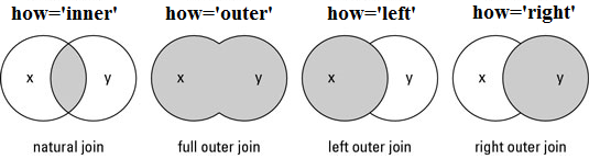
Fig. 38 Visualization for the four main ways to merge, or join, data.#
We will use pd.join to do this. I’m going to bring in two sets of data from CRSP. Each data set has the same three securities, XOM, AAPL, and TLT, over the same time period (Jan 2019 - Dec 2021). But, they have some different variables.
crsp1 = pd.read_csv('https://raw.githubusercontent.com/aaiken1/fin-data-analysis-python/main/data/crsp_022722.csv')
crsp2 = pd.read_csv('https://raw.githubusercontent.com/aaiken1/fin-data-analysis-python/main/data/crsp_030622.csv')
We can look at each DataFrame and see what they have.
crsp1
| PERMNO | date | TICKER | CUSIP | DISTCD | DIVAMT | FACPR | FACSHR | PRC | VOL | RET | SHROUT | CFACPR | CFACSHR | sprtrn | |
|---|---|---|---|---|---|---|---|---|---|---|---|---|---|---|---|
| 0 | 11850 | 20190102 | XOM | 30231G10 | NaN | NaN | NaN | NaN | 69.69000 | 16727246 | 0.021997 | 4233807 | 1 | 1 | 0.001269 |
| 1 | 11850 | 20190103 | XOM | 30231G10 | NaN | NaN | NaN | NaN | 68.62000 | 13866115 | -0.015354 | 4233807 | 1 | 1 | -0.024757 |
| 2 | 11850 | 20190104 | XOM | 30231G10 | NaN | NaN | NaN | NaN | 71.15000 | 16043642 | 0.036870 | 4233807 | 1 | 1 | 0.034336 |
| 3 | 11850 | 20190107 | XOM | 30231G10 | NaN | NaN | NaN | NaN | 71.52000 | 10844159 | 0.005200 | 4233807 | 1 | 1 | 0.007010 |
| 4 | 11850 | 20190108 | XOM | 30231G10 | NaN | NaN | NaN | NaN | 72.04000 | 11438966 | 0.007271 | 4233807 | 1 | 1 | 0.009695 |
| ... | ... | ... | ... | ... | ... | ... | ... | ... | ... | ... | ... | ... | ... | ... | ... |
| 2266 | 89468 | 20211227 | TLT | 46428743 | NaN | NaN | NaN | NaN | 148.88000 | 7854290 | 0.002424 | 132000 | 1 | 1 | 0.013839 |
| 2267 | 89468 | 20211228 | TLT | 46428743 | NaN | NaN | NaN | NaN | 148.28999 | 9173504 | -0.003963 | 133200 | 1 | 1 | -0.001010 |
| 2268 | 89468 | 20211229 | TLT | 46428743 | NaN | NaN | NaN | NaN | 146.67000 | 11763496 | -0.010925 | 133400 | 1 | 1 | 0.001402 |
| 2269 | 89468 | 20211230 | TLT | 46428743 | NaN | NaN | NaN | NaN | 147.89999 | 10340148 | 0.008386 | 133400 | 1 | 1 | -0.002990 |
| 2270 | 89468 | 20211231 | TLT | 46428743 | NaN | NaN | NaN | NaN | 148.19000 | 13389734 | 0.001961 | 132800 | 1 | 1 | -0.002626 |
2271 rows × 15 columns
crsp2
| PERMNO | date | TICKER | COMNAM | CUSIP | RETX | |
|---|---|---|---|---|---|---|
| 0 | 11850 | 20190102 | XOM | EXXON MOBIL CORP | 30231G10 | 0.021997 |
| 1 | 11850 | 20190103 | XOM | EXXON MOBIL CORP | 30231G10 | -0.015354 |
| 2 | 11850 | 20190104 | XOM | EXXON MOBIL CORP | 30231G10 | 0.036870 |
| 3 | 11850 | 20190107 | XOM | EXXON MOBIL CORP | 30231G10 | 0.005200 |
| 4 | 11850 | 20190108 | XOM | EXXON MOBIL CORP | 30231G10 | 0.007271 |
| ... | ... | ... | ... | ... | ... | ... |
| 2266 | 89468 | 20211227 | TLT | ISHARES TRUST | 46428743 | 0.002424 |
| 2267 | 89468 | 20211228 | TLT | ISHARES TRUST | 46428743 | -0.003963 |
| 2268 | 89468 | 20211229 | TLT | ISHARES TRUST | 46428743 | -0.010925 |
| 2269 | 89468 | 20211230 | TLT | ISHARES TRUST | 46428743 | 0.008386 |
| 2270 | 89468 | 20211231 | TLT | ISHARES TRUST | 46428743 | 0.001961 |
2271 rows × 6 columns
We can see that they each have the same IDs (e.g. PERMNO) and date. The crsp2 DataFrame has an additional variable, RETX, or returns without dividends, that I want to merge in. I’m going to simplify the crsp2 DataFrame and only keep three variables: PERMNO, date, and retx. I will then merge using PERMNO and date as my keys. These two variables uniquely identify each row.
I will do an inner join. This will only keep PERMNO-date observations that are in both data sets. An outer join would keep all observations, including those that are in one dataset, but not the other. This might be helpful if you had PERMNOs in one data set, but not the other, and you wanted to keep all of your data.
For this particular data, there should be a 1:1 correspondence between the observations.
crsp2_clean = crsp2[['PERMNO', 'date', 'RETX']]
merged = crsp1.merge(crsp2_clean, how = 'inner', on = ['PERMNO', 'date'] )
merged
| PERMNO | date | TICKER | CUSIP | DISTCD | DIVAMT | FACPR | FACSHR | PRC | VOL | RET | SHROUT | CFACPR | CFACSHR | sprtrn | RETX | |
|---|---|---|---|---|---|---|---|---|---|---|---|---|---|---|---|---|
| 0 | 11850 | 20190102 | XOM | 30231G10 | NaN | NaN | NaN | NaN | 69.69000 | 16727246 | 0.021997 | 4233807 | 1 | 1 | 0.001269 | 0.021997 |
| 1 | 11850 | 20190103 | XOM | 30231G10 | NaN | NaN | NaN | NaN | 68.62000 | 13866115 | -0.015354 | 4233807 | 1 | 1 | -0.024757 | -0.015354 |
| 2 | 11850 | 20190104 | XOM | 30231G10 | NaN | NaN | NaN | NaN | 71.15000 | 16043642 | 0.036870 | 4233807 | 1 | 1 | 0.034336 | 0.036870 |
| 3 | 11850 | 20190107 | XOM | 30231G10 | NaN | NaN | NaN | NaN | 71.52000 | 10844159 | 0.005200 | 4233807 | 1 | 1 | 0.007010 | 0.005200 |
| 4 | 11850 | 20190108 | XOM | 30231G10 | NaN | NaN | NaN | NaN | 72.04000 | 11438966 | 0.007271 | 4233807 | 1 | 1 | 0.009695 | 0.007271 |
| ... | ... | ... | ... | ... | ... | ... | ... | ... | ... | ... | ... | ... | ... | ... | ... | ... |
| 2266 | 89468 | 20211227 | TLT | 46428743 | NaN | NaN | NaN | NaN | 148.88000 | 7854290 | 0.002424 | 132000 | 1 | 1 | 0.013839 | 0.002424 |
| 2267 | 89468 | 20211228 | TLT | 46428743 | NaN | NaN | NaN | NaN | 148.28999 | 9173504 | -0.003963 | 133200 | 1 | 1 | -0.001010 | -0.003963 |
| 2268 | 89468 | 20211229 | TLT | 46428743 | NaN | NaN | NaN | NaN | 146.67000 | 11763496 | -0.010925 | 133400 | 1 | 1 | 0.001402 | -0.010925 |
| 2269 | 89468 | 20211230 | TLT | 46428743 | NaN | NaN | NaN | NaN | 147.89999 | 10340148 | 0.008386 | 133400 | 1 | 1 | -0.002990 | 0.008386 |
| 2270 | 89468 | 20211231 | TLT | 46428743 | NaN | NaN | NaN | NaN | 148.19000 | 13389734 | 0.001961 | 132800 | 1 | 1 | -0.002626 | 0.001961 |
2271 rows × 16 columns
You can see the RETX variable at the end of the merged DataFrame.
What happens if you don’t clean up with crsp2 data first?
merged = crsp1.merge(crsp2, how = 'inner', on = ['PERMNO', 'date'] )
merged
| PERMNO | date | TICKER_x | CUSIP_x | DISTCD | DIVAMT | FACPR | FACSHR | PRC | VOL | RET | SHROUT | CFACPR | CFACSHR | sprtrn | TICKER_y | COMNAM | CUSIP_y | RETX | |
|---|---|---|---|---|---|---|---|---|---|---|---|---|---|---|---|---|---|---|---|
| 0 | 11850 | 20190102 | XOM | 30231G10 | NaN | NaN | NaN | NaN | 69.69000 | 16727246 | 0.021997 | 4233807 | 1 | 1 | 0.001269 | XOM | EXXON MOBIL CORP | 30231G10 | 0.021997 |
| 1 | 11850 | 20190103 | XOM | 30231G10 | NaN | NaN | NaN | NaN | 68.62000 | 13866115 | -0.015354 | 4233807 | 1 | 1 | -0.024757 | XOM | EXXON MOBIL CORP | 30231G10 | -0.015354 |
| 2 | 11850 | 20190104 | XOM | 30231G10 | NaN | NaN | NaN | NaN | 71.15000 | 16043642 | 0.036870 | 4233807 | 1 | 1 | 0.034336 | XOM | EXXON MOBIL CORP | 30231G10 | 0.036870 |
| 3 | 11850 | 20190107 | XOM | 30231G10 | NaN | NaN | NaN | NaN | 71.52000 | 10844159 | 0.005200 | 4233807 | 1 | 1 | 0.007010 | XOM | EXXON MOBIL CORP | 30231G10 | 0.005200 |
| 4 | 11850 | 20190108 | XOM | 30231G10 | NaN | NaN | NaN | NaN | 72.04000 | 11438966 | 0.007271 | 4233807 | 1 | 1 | 0.009695 | XOM | EXXON MOBIL CORP | 30231G10 | 0.007271 |
| ... | ... | ... | ... | ... | ... | ... | ... | ... | ... | ... | ... | ... | ... | ... | ... | ... | ... | ... | ... |
| 2266 | 89468 | 20211227 | TLT | 46428743 | NaN | NaN | NaN | NaN | 148.88000 | 7854290 | 0.002424 | 132000 | 1 | 1 | 0.013839 | TLT | ISHARES TRUST | 46428743 | 0.002424 |
| 2267 | 89468 | 20211228 | TLT | 46428743 | NaN | NaN | NaN | NaN | 148.28999 | 9173504 | -0.003963 | 133200 | 1 | 1 | -0.001010 | TLT | ISHARES TRUST | 46428743 | -0.003963 |
| 2268 | 89468 | 20211229 | TLT | 46428743 | NaN | NaN | NaN | NaN | 146.67000 | 11763496 | -0.010925 | 133400 | 1 | 1 | 0.001402 | TLT | ISHARES TRUST | 46428743 | -0.010925 |
| 2269 | 89468 | 20211230 | TLT | 46428743 | NaN | NaN | NaN | NaN | 147.89999 | 10340148 | 0.008386 | 133400 | 1 | 1 | -0.002990 | TLT | ISHARES TRUST | 46428743 | 0.008386 |
| 2270 | 89468 | 20211231 | TLT | 46428743 | NaN | NaN | NaN | NaN | 148.19000 | 13389734 | 0.001961 | 132800 | 1 | 1 | -0.002626 | TLT | ISHARES TRUST | 46428743 | 0.001961 |
2271 rows × 19 columns
Do you see the _x and _y suffixes? pd.merge adds that when you have two variables with the same name in both data sets that you are not using as key values. The variables that you merge on, the key values, truly get merged together, and so you only get one column for PERMNO and one column for date, in this example. But, TICKER is in both data sets and is not a key value. So, when you merge the data, you’re going to have two columns names TICKER. The _x means that the variable is from the left (first) data set and the _y means that the variable is from the right (second) data set.
You can read more about pd.merge here. Bad merges that lose observations are a common problem.
You have to understand your data structure before trying to combine DataFrames together.
Multiple Levels#
So far, we’ve only defined data with one index value, like a date or a stock ticker. But - look at the return data above. There is both a stock and a date. When data has an ID and a time dimension, we call that panel data. For example, stock-level or firm-level data through time. pandas can help us deal with this type of data as well.
You can read more about MultiIndex data on the pandas help page.
This type of data is also called hierarchical. Let’s use the crsp2 DataFrame to see what’s going on.
crsp2
| PERMNO | date | TICKER | COMNAM | CUSIP | RETX | |
|---|---|---|---|---|---|---|
| 0 | 11850 | 20190102 | XOM | EXXON MOBIL CORP | 30231G10 | 0.021997 |
| 1 | 11850 | 20190103 | XOM | EXXON MOBIL CORP | 30231G10 | -0.015354 |
| 2 | 11850 | 20190104 | XOM | EXXON MOBIL CORP | 30231G10 | 0.036870 |
| 3 | 11850 | 20190107 | XOM | EXXON MOBIL CORP | 30231G10 | 0.005200 |
| 4 | 11850 | 20190108 | XOM | EXXON MOBIL CORP | 30231G10 | 0.007271 |
| ... | ... | ... | ... | ... | ... | ... |
| 2266 | 89468 | 20211227 | TLT | ISHARES TRUST | 46428743 | 0.002424 |
| 2267 | 89468 | 20211228 | TLT | ISHARES TRUST | 46428743 | -0.003963 |
| 2268 | 89468 | 20211229 | TLT | ISHARES TRUST | 46428743 | -0.010925 |
| 2269 | 89468 | 20211230 | TLT | ISHARES TRUST | 46428743 | 0.008386 |
| 2270 | 89468 | 20211231 | TLT | ISHARES TRUST | 46428743 | 0.001961 |
2271 rows × 6 columns
We have PERMNO, our ID, and date. Together, these each define a unique observation.
We can see that crsp2 doesn’t have an index that we’ve defined. It is just the default number.
crsp2.index
RangeIndex(start=0, stop=2271, step=1)
I’ll now set two indices for the CRSP data and save this as a new DataFrame called crsp3. I’m using the pandas .set_index() function and
passing the name of the columns in the list.
I then sort the data using .sort_index(). This does what it says - it sorts by date and then PERMNO.
crsp3 = crsp2.set_index(['date', 'PERMNO'])

crsp3.sort_index()

crsp3
| TICKER | COMNAM | CUSIP | RETX | ||
|---|---|---|---|---|---|
| date | PERMNO | ||||
| 20190102 | 11850 | XOM | EXXON MOBIL CORP | 30231G10 | 0.021997 |
| 20190103 | 11850 | XOM | EXXON MOBIL CORP | 30231G10 | -0.015354 |
| 20190104 | 11850 | XOM | EXXON MOBIL CORP | 30231G10 | 0.036870 |
| 20190107 | 11850 | XOM | EXXON MOBIL CORP | 30231G10 | 0.005200 |
| 20190108 | 11850 | XOM | EXXON MOBIL CORP | 30231G10 | 0.007271 |
| ... | ... | ... | ... | ... | ... |
| 20211227 | 89468 | TLT | ISHARES TRUST | 46428743 | 0.002424 |
| 20211228 | 89468 | TLT | ISHARES TRUST | 46428743 | -0.003963 |
| 20211229 | 89468 | TLT | ISHARES TRUST | 46428743 | -0.010925 |
| 20211230 | 89468 | TLT | ISHARES TRUST | 46428743 | 0.008386 |
| 20211231 | 89468 | TLT | ISHARES TRUST | 46428743 | 0.001961 |
2271 rows × 4 columns
You can see the multiple levels now. You can perform operations by using these indices.
Let’s group by PERMNO, or our Level 1 index, and calculate the average return for each stock across all dates.
crsp3.groupby(level = 1)['RETX'].mean()
PERMNO
11850    0.000124
14593    0.002221
89468    0.000315
Name: RETX, dtype: float64
Let’s do the same thing using the first level, or the date. This gives the average return of the three stocks on each date.
crsp3.groupby(level = 0)['RETX'].mean()
date
20190102    0.009468
20190103   -0.034527
20190104    0.022661
20190107    0.000009
20190108    0.007902
              ...
20211227    0.013219
20211228   -0.004321
20211229   -0.006392
20211230   -0.001360
20211231    0.001669
Name: RETX, Length: 757, dtype: float64
As before, we can use to.frame() to go from a series to a DataFrame and make the output look a little nicer.
crsp3.groupby(level = 1)['RETX'].mean().to_frame()
| RETX | |
|---|---|
| PERMNO | |
| 11850 | 0.000124 |
| 14593 | 0.002221 |
| 89468 | 0.000315 |
We can use the name of the levels, too. Here I’ll find the min and the max return for each stock and save it as a new DataFrame.
crsp3_agg = crsp3.groupby(level = ['PERMNO'])['RETX'].agg(['max', 'min'])
crsp3_agg
| max | min | |
|---|---|---|
| PERMNO | ||
| 11850 | 0.126868 | -0.122248 |
| 14593 | 0.119808 | -0.128647 |
| 89468 | 0.075196 | -0.066683 |
With indices defined, I can use .unstack() to from long to wide data. I’ll take the return and create new columns for each stock.
crsp3['RETX'].unstack()
| PERMNO | 11850 | 14593 | 89468 |
|---|---|---|---|
| date | |||
| 20190102 | 0.021997 | 0.001141 | 0.005267 |
| 20190103 | -0.015354 | -0.099607 | 0.011379 |
| 20190104 | 0.036870 | 0.042689 | -0.011575 |
| 20190107 | 0.005200 | -0.002226 | -0.002948 |
| 20190108 | 0.007271 | 0.019063 | -0.002628 |
| ... | ... | ... | ... |
| 20211227 | 0.014258 | 0.022975 | 0.002424 |
| 20211228 | -0.003232 | -0.005767 | -0.003963 |
| 20211229 | -0.008753 | 0.000502 | -0.010925 |
| 20211230 | -0.005887 | -0.006578 | 0.008386 |
| 20211231 | 0.006580 | -0.003535 | 0.001961 |
757 rows × 3 columns
Note
The PERMNOs are now the column headers, so we’re treating each stock like a variable. You’ll see a lot of finance data like this, with tickers or another ID as columns. But, you can no longer merge on the stock if you wanted to bring in additional variables! This is why the organization of your data is so important. Long data is easier to deal with when combining data sets.
If I had defined the PERMNO as the Level 0 index and date as the Level 1 index, then I would have unstacked my data with dates as the columns and the stocks as the rows. That’s not what I wanted, though.
Columns and levels#
The unstacked data above has a PERMNO for each column. Underneath each PERMNO is a return. But, what if we have, say, both return and price data?
We can also add levels to our columns, creating groups of variables when we have wide data. Let’s go back to the wide3 DataFrame from above. We can also go even wider. Let’s get of the two indices, PERMNO and date, in wide3 and turn them both back into columns.
wide3 = wide3.reset_index()
wide3
| vars | PERMNO | date | PRC | RET |
|---|---|---|---|---|
| 0 | 10107 | 20190513 | 123.35000 | -0.029733 |
| 1 | 11850 | 20190513 | 75.71000 | -0.011102 |
| 2 | 14593 | 20190513 | 185.72000 | -0.058119 |
| 3 | 93436 | 20190513 | 227.00999 | -0.052229 |
Now, let’s create a DataFrame where just date is an index and go wider, where each column is now either a RET or a PRC for each PERMNO.
wide4 = pd.pivot(wide3, values = ['RET', 'PRC'], columns = 'PERMNO', index = 'date')
wide4
| RET | PRC | |||||||
|---|---|---|---|---|---|---|---|---|
| PERMNO | 10107 | 11850 | 14593 | 93436 | 10107 | 11850 | 14593 | 93436 |
| date | ||||||||
| 20190513 | -0.029733 | -0.011102 | -0.058119 | -0.052229 | 123.35 | 75.71 | 185.72 | 227.00999 |
We only had one date, so this isn’t a very interesting DataFrame.
I can take my DataFrame, select the index, and get the name of my index. Remember, indices are about the rows.
wide4.index.names
FrozenList(['date'])
But, you can tell from the above DataFrame that my columns now look different. They have what pandas calls levels.
wide4.columns.levels
FrozenList([['RET', 'PRC'], [10107, 11850, 14593, 93436]])
See how there are two lists? One for each level of column.
Preview: Calculating Returns#
Now that you know how to reshape data and work with multiple securities, you’re ready for financial calculations. One method you’ll use constantly is .pct_change(), which calculates percentage changes between rows - exactly what you need for returns.
Here’s a quick preview:
# If you have prices, you can calculate returns with pct_change()
aapl['return_calc'] = aapl['PRC'].pct_change()
aapl[['PRC', 'RET', 'return_calc']].head()
| PRC | RET | return_calc | |
|---|---|---|---|
| date | |||
| 20190102 | 157.92000 | 0.001141 | NaN |
| 20190103 | 142.19000 | -0.099607 | -0.099607 |
| 20190104 | 148.25999 | 0.042689 | 0.042689 |
| 20190107 | 147.92999 | -0.002226 | -0.002226 |
| 20190108 | 150.75000 | 0.019063 | 0.019063 |
The .pct_change() method calculates (current - previous) / previous - exactly the formula for a simple return. Notice how the first row is NaN? That’s because there’s no previous price to compare to.
We’ll use .pct_change() extensively when we get to financial time series and portfolio math. For now, just know it exists and that pandas makes return calculations easy.