
Financial time series #
Python and, in particular, pandas can easily deal with the most common type of financial data - time series data. We are going to look at the basics of using price and return data. This section follows Chapter 8 of Python for Finance, 2e and pieces of a DataCamp assignment that I’ve used in previous years.
A time series is a dataset where values are recorded over time at regular intervals (e.g., daily stock prices, quarterly GDP, or annual revenue). In finance, time series data is used to analyze trends, volatility, and seasonality in stock prices, returns, and macroeconomic indicators.
We’ll cover importing time series data and getting some summary statistics, as well as return calculations, resampling, or changing the periodicity of the data (i.e. going from daily to monthly to annual), and rolling statistics, such as finding moving averages and other statistics over rolling windows (e.g. one month of trading days).
Time series data means handling dates. There is a DataCamp tutorial on datetime objects.
We’ll start with the usual sort of set-up and our familiar stock data. Our data is going to have a particular set-up in this section. Each column is going to represent both a security and something about that security. So, Apple’s price. Or, Apple’s return. This is a very common way to see financial data, but it is not the only way that this data can be organized.
Set-up and descriptives#
# Set-up

import numpy as np
import pandas as pd

# Date functionality
from datetime import datetime
from datetime import timedelta

import janitor
from janitor import clean_names

# all of matplotlib
import matplotlib as mpl

# refer to the pyplot part of matplot lib more easily. Just use plt!
import matplotlib.pyplot as plt

# importing the style package
from matplotlib import style
from matplotlib.ticker import StrMethodFormatter

# generating random numbers
from numpy.random import normal, seed
from scipy.stats import norm

# seaborn
import seaborn as sns

# Keeps warnings from cluttering up our notebook.
import warnings
warnings.filterwarnings('ignore')

# Include this to have plots show up in your Jupyter notebook.
%matplotlib inline

# Some plot options that will apply to the whole workbook
plt.style.use('seaborn-v0_8')
mpl.rcParams['font.family'] = 'serif'


# Read in some eod prices
stocks = pd.read_csv('https://raw.githubusercontent.com/aaiken1/fin-data-analysis-python/main/data/tr_eikon_eod_data.csv',
                  index_col=0, parse_dates=True)

stocks = stocks.dropna()

stocks = clean_names(stocks)

stocks.info()
<class 'pandas.core.frame.DataFrame'>
DatetimeIndex: 2138 entries, 2010-01-04 to 2018-06-29
Data columns (total 12 columns):
 #   Column  Non-Null Count  Dtype
---  ------  --------------  -----
 0   aapl_o  2138 non-null   float64
 1   msft_o  2138 non-null   float64
 2   intc_o  2138 non-null   float64
 3   amzn_o  2138 non-null   float64
 4   gs_n    2138 non-null   float64
 5   spy     2138 non-null   float64
 6   _spx    2138 non-null   float64
 7   _vix    2138 non-null   float64
 8   eur=    2138 non-null   float64
 9   xau=    2138 non-null   float64
 10  gdx     2138 non-null   float64
 11  gld     2138 non-null   float64
dtypes: float64(12)
memory usage: 217.1 KB
We are using pandas DataFrames, which have many built-in ways to deal with time series data. We have made our index the date. This is important - having the date be our index opens up various date-related methods.
Parsing dates when you import the data is faster than doing it after loading, if you’re dealing with large data sets.
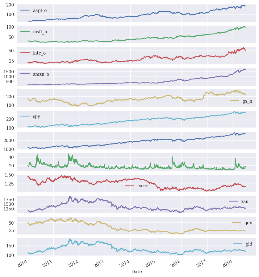
Let’s use pandas plot to make a quick figure of all of the prices over the time period in our data. Remember, pandas has its own plotting functions. They are very useful for quick plots like this. Because the date is our index, pandas knows to put that on the x-axis, right where we want it.
stocks.plot(figsize=(10, 12), subplots=True);
We can use .describe() to look at our prices.
stocks.describe().round(2)
| aapl_o | msft_o | intc_o | amzn_o | gs_n | spy | _spx | _vix | eur= | xau= | gdx | gld | |
|---|---|---|---|---|---|---|---|---|---|---|---|---|
| count | 2138.00 | 2138.00 | 2138.00 | 2138.00 | 2138.00 | 2138.00 | 2138.00 | 2138.00 | 2138.00 | 2138.00 | 2138.00 | 2138.00 |
| mean | 93.46 | 44.56 | 29.36 | 480.46 | 170.22 | 180.32 | 1802.71 | 17.03 | 1.25 | 1348.91 | 33.57 | 130.09 |
| std | 40.55 | 19.53 | 8.17 | 372.31 | 42.48 | 48.19 | 483.34 | 5.88 | 0.11 | 188.21 | 15.17 | 18.78 |
| min | 27.44 | 23.01 | 17.66 | 108.61 | 87.70 | 102.20 | 1022.58 | 9.14 | 1.04 | 1051.36 | 12.47 | 100.50 |
| 25% | 60.29 | 28.57 | 22.51 | 213.60 | 146.61 | 133.99 | 1338.57 | 13.07 | 1.13 | 1222.49 | 22.14 | 117.40 |
| 50% | 90.55 | 39.66 | 27.33 | 322.06 | 164.43 | 186.32 | 1863.08 | 15.58 | 1.27 | 1292.68 | 25.62 | 124.00 |
| 75% | 117.24 | 54.37 | 34.71 | 698.85 | 192.13 | 210.99 | 2108.94 | 19.07 | 1.35 | 1427.57 | 48.34 | 139.00 |
| max | 193.98 | 102.49 | 57.08 | 1750.08 | 273.38 | 286.58 | 2872.87 | 48.00 | 1.48 | 1897.10 | 66.63 | 184.59 |
We can use .aggregate() to create our own set of descriptives.
stocks.aggregate([min,
                np.mean,
                np.std,
                np.median,
                max]
).round(2)
| aapl_o | msft_o | intc_o | amzn_o | gs_n | spy | _spx | _vix | eur= | xau= | gdx | gld | |
|---|---|---|---|---|---|---|---|---|---|---|---|---|
| min | 27.44 | 23.01 | 17.66 | 108.61 | 87.70 | 102.20 | 1022.58 | 9.14 | 1.04 | 1051.36 | 12.47 | 100.50 |
| mean | 93.46 | 44.56 | 29.36 | 480.46 | 170.22 | 180.32 | 1802.71 | 17.03 | 1.25 | 1348.91 | 33.57 | 130.09 |
| std | 40.55 | 19.53 | 8.17 | 372.31 | 42.48 | 48.19 | 483.34 | 5.88 | 0.11 | 188.21 | 15.17 | 18.78 |
| median | 90.55 | 39.66 | 27.33 | 322.06 | 164.43 | 186.32 | 1863.08 | 15.58 | 1.27 | 1292.68 | 25.62 | 124.00 |
| max | 193.98 | 102.49 | 57.08 | 1750.08 | 273.38 | 286.58 | 2872.87 | 48.00 | 1.48 | 1897.10 | 66.63 | 184.59 |
Dates#
Obviously, we need to handle a variety of time periods in finance. Two libraries are being used here: datetime and pandas. We can use pandas to objects and methods that help us deal with dates.
We can define a TimeStamp and see that they are a particular object-type in Python. All objects come with methods and attributes. This is a generic idea from computer science called object oriented programming.
In Python, dates can be stored as strings (e.g., "2024-01-01") or as date objects (e.g., datetime.datetime(2024, 1, 1)).
For time series analysis, we need to ensure our dates are in the correct format so that:
They can be sorted chronologically.
We can perform resampling (e.g., converting daily data to monthly).
We can easily calculate time-based differences.
my_date = pd.Timestamp(datetime(2022, 2, 23))
print(type(my_date))
my_date
<class 'pandas._libs.tslibs.timestamps.Timestamp'>
Timestamp('2022-02-23 00:00:00')
Here’s an example of an attribute for a TimeStamp object. You can also do .month, .day, .dayofweek, etc.
my_date.year
2022
We can add and subtract with dates using timedelta. Note that datetime no longer wants you to just add or subtract a number from a date.
There’s both a datetime timedelta and a pandas Timedelta. You can read about the pandas version here.
my_date + timedelta(days=7)
Timestamp('2022-03-02 00:00:00')
Using the pandas version, just to highlight that different libraries have similar functionality. The datetime library and the pandas library are different things. But, they can do similar operations with time, even if the syntax varies a bit.
my_date + pd.Timedelta(7, "d")
Timestamp('2022-03-02 00:00:00')
pandas has a set of tools related to a period in time. You can define a period, get attributes, and change its frequency. Changing the frequency means changing how pandas thinks about the period. Is this month? Is this a particular day?
Let’s define a period as February 2022.
period = pd.Period('2022-02')
period
Period('2022-02', 'M')
We can then change that to a daily frequency. Note how, by default, pandas puts us at the end of the month.
period.asfreq('D')
Period('2022-02-28', 'D')
This can be really helpful when some Excel data comes in as, say “May-2019” and we want to get that to be an end of month date, like “5/31/19”. The actual day is ambiguous when just dealing with month and year.
With the date as our index, we can pull certain dates and columns. Here’s Apple’s price on 2017-6-1.
stocks.loc['2017-6-1', 'aapl_o']
153.18
Here’s all of the columns, but just for a subset of dates.
stocks.loc['2015-3':'2016-2',:]
| aapl_o | msft_o | intc_o | amzn_o | gs_n | spy | _spx | _vix | eur= | xau= | gdx | gld | |
|---|---|---|---|---|---|---|---|---|---|---|---|---|
| Date | ||||||||||||
| 2015-03-02 | 129.09 | 43.880 | 34.060 | 385.655 | 191.79 | 211.9900 | 2117.39 | 13.04 | 1.1183 | 1206.70 | 20.76 | 115.68 |
| 2015-03-03 | 129.36 | 43.280 | 34.095 | 384.610 | 191.27 | 211.1200 | 2107.78 | 13.86 | 1.1174 | 1203.31 | 20.38 | 115.47 |
| 2015-03-04 | 128.54 | 43.055 | 34.120 | 382.720 | 189.67 | 210.2301 | 2098.53 | 14.23 | 1.1077 | 1199.45 | 20.04 | 115.11 |
| 2015-03-05 | 126.41 | 43.110 | 33.730 | 387.830 | 190.08 | 210.4600 | 2101.04 | 14.04 | 1.1028 | 1198.20 | 20.08 | 115.00 |
| 2015-03-06 | 126.60 | 42.360 | 33.190 | 380.090 | 186.91 | 207.5000 | 2071.26 | 15.20 | 1.0843 | 1166.72 | 18.58 | 111.86 |
| ... | ... | ... | ... | ... | ... | ... | ... | ... | ... | ... | ... | ... |
| 2016-02-23 | 94.69 | 51.180 | 28.800 | 552.940 | 144.91 | 192.3200 | 1921.27 | 20.98 | 1.1017 | 1227.06 | 18.92 | 117.22 |
| 2016-02-24 | 96.10 | 51.360 | 29.190 | 554.040 | 145.56 | 193.2000 | 1929.80 | 20.72 | 1.1011 | 1228.96 | 19.11 | 117.61 |
| 2016-02-25 | 96.76 | 52.100 | 29.620 | 555.150 | 148.25 | 195.5400 | 1951.70 | 19.11 | 1.1021 | 1234.26 | 19.39 | 117.92 |
| 2016-02-26 | 96.91 | 51.300 | 29.800 | 555.230 | 150.25 | 195.0892 | 1948.05 | 19.81 | 1.0931 | 1222.21 | 18.69 | 117.11 |
| 2016-02-29 | 96.69 | 50.880 | 29.590 | 552.520 | 149.53 | 193.5600 | 1932.23 | 20.55 | 1.0871 | 1237.76 | 19.38 | 118.64 |
252 rows × 12 columns
Calculating returns#
We can start by just calculating the price change from day-to-day using pandas diff(). This function is described here. Notice how the first day in the data is now NaN, since you can’t calculate a change without the previous day.
Since there’s no =, I am not saving the data. Just showing you what the function does.
stocks.diff().head()
| aapl_o | msft_o | intc_o | amzn_o | gs_n | spy | _spx | _vix | eur= | xau= | gdx | gld | |
|---|---|---|---|---|---|---|---|---|---|---|---|---|
| Date | ||||||||||||
| 2010-01-04 | NaN | NaN | NaN | NaN | NaN | NaN | NaN | NaN | NaN | NaN | NaN | NaN |
| 2010-01-05 | 0.052857 | 0.010 | -0.01 | 0.79 | 3.06 | 0.30 | 3.53 | -0.69 | -0.0043 | -1.35 | 0.46 | -0.10 |
| 2010-01-06 | -0.487142 | -0.190 | -0.07 | -2.44 | -1.88 | 0.08 | 0.62 | -0.19 | 0.0044 | 19.85 | 1.17 | 1.81 |
| 2010-01-07 | -0.055714 | -0.318 | -0.20 | -2.25 | 3.41 | 0.48 | 4.55 | -0.10 | -0.0094 | -6.60 | -0.24 | -0.69 |
| 2010-01-08 | 0.200000 | 0.208 | 0.23 | 3.52 | -3.36 | 0.38 | 3.29 | -0.93 | 0.0094 | 4.20 | 0.74 | 0.55 |
Sometimes we want price changes. Other times we want pandas pct_change(). See this for more. This function allows us to calculate price returns using the percent change. The default is to look back one period, or one day in this case.
stocks.pct_change().mul(100).round(3).head()
| aapl_o | msft_o | intc_o | amzn_o | gs_n | spy | _spx | _vix | eur= | xau= | gdx | gld | |
|---|---|---|---|---|---|---|---|---|---|---|---|---|
| Date | ||||||||||||
| 2010-01-04 | NaN | NaN | NaN | NaN | NaN | NaN | NaN | NaN | NaN | NaN | NaN | NaN |
| 2010-01-05 | 0.173 | 0.032 | -0.048 | 0.590 | 1.768 | 0.265 | 0.312 | -3.443 | -0.298 | -0.121 | 0.964 | -0.091 |
| 2010-01-06 | -1.591 | -0.614 | -0.335 | -1.812 | -1.067 | 0.070 | 0.055 | -0.982 | 0.306 | 1.774 | 2.429 | 1.650 |
| 2010-01-07 | -0.185 | -1.033 | -0.962 | -1.701 | 1.957 | 0.422 | 0.400 | -0.522 | -0.652 | -0.580 | -0.486 | -0.619 |
| 2010-01-08 | 0.665 | 0.683 | 1.117 | 2.708 | -1.891 | 0.333 | 0.288 | -4.879 | 0.657 | 0.371 | 1.507 | 0.496 |
I’m multiplying by 100 just for the display of the data.
The percent change is called a linear return. Or, simple return. This is different from log returns, or compounded returns. Both types of returns are correct and useful. They are just used for different things.
The formula for simple returns (R) is:
where R is the simple return based on the percent change and V is the cash flow, including price and dividends (if any).
The formula for log returns (r) is:
See this article for more on why this difference is important. In short, we need the mean of simple returns when doing portfolio optimization, as these returns work with a weighted average. Simple returns aggregate across assets. Log returns, however, aggregate across time. In other words, the cumulative return using log returns is the sum of individual log returns over the time period. You definitely can’t do that with simple returns!
Here’s a brief video that describes the same thing using Excel.
Finally, this chapter has everything you’ve ever want to know about return calculations. See pgs. 16 and 17 for log returns.
We can calculate log returns using np.log and .shift() from pandas. Let’s look at what .shift() does. Compare the following:
stocks
| aapl_o | msft_o | intc_o | amzn_o | gs_n | spy | _spx | _vix | eur= | xau= | gdx | gld | |
|---|---|---|---|---|---|---|---|---|---|---|---|---|
| Date | ||||||||||||
| 2010-01-04 | 30.572827 | 30.950 | 20.88 | 133.90 | 173.08 | 113.33 | 1132.99 | 20.04 | 1.4411 | 1120.00 | 47.71 | 109.80 |
| 2010-01-05 | 30.625684 | 30.960 | 20.87 | 134.69 | 176.14 | 113.63 | 1136.52 | 19.35 | 1.4368 | 1118.65 | 48.17 | 109.70 |
| 2010-01-06 | 30.138541 | 30.770 | 20.80 | 132.25 | 174.26 | 113.71 | 1137.14 | 19.16 | 1.4412 | 1138.50 | 49.34 | 111.51 |
| 2010-01-07 | 30.082827 | 30.452 | 20.60 | 130.00 | 177.67 | 114.19 | 1141.69 | 19.06 | 1.4318 | 1131.90 | 49.10 | 110.82 |
| 2010-01-08 | 30.282827 | 30.660 | 20.83 | 133.52 | 174.31 | 114.57 | 1144.98 | 18.13 | 1.4412 | 1136.10 | 49.84 | 111.37 |
| ... | ... | ... | ... | ... | ... | ... | ... | ... | ... | ... | ... | ... |
| 2018-06-25 | 182.170000 | 98.390 | 50.71 | 1663.15 | 221.54 | 271.00 | 2717.07 | 17.33 | 1.1702 | 1265.00 | 22.01 | 119.89 |
| 2018-06-26 | 184.430000 | 99.080 | 49.67 | 1691.09 | 221.58 | 271.60 | 2723.06 | 15.92 | 1.1645 | 1258.64 | 21.95 | 119.26 |
| 2018-06-27 | 184.160000 | 97.540 | 48.76 | 1660.51 | 220.18 | 269.35 | 2699.63 | 17.91 | 1.1552 | 1251.62 | 21.81 | 118.58 |
| 2018-06-28 | 185.500000 | 98.630 | 49.25 | 1701.45 | 223.42 | 270.89 | 2716.31 | 16.85 | 1.1567 | 1247.88 | 21.93 | 118.22 |
| 2018-06-29 | 185.110000 | 98.610 | 49.71 | 1699.80 | 220.57 | 271.28 | 2718.37 | 16.09 | 1.1683 | 1252.25 | 22.31 | 118.65 |
2138 rows × 12 columns
stocks.shift(1)
| aapl_o | msft_o | intc_o | amzn_o | gs_n | spy | _spx | _vix | eur= | xau= | gdx | gld | |
|---|---|---|---|---|---|---|---|---|---|---|---|---|
| Date | ||||||||||||
| 2010-01-04 | NaN | NaN | NaN | NaN | NaN | NaN | NaN | NaN | NaN | NaN | NaN | NaN |
| 2010-01-05 | 30.572827 | 30.950 | 20.88 | 133.90 | 173.08 | 113.33 | 1132.99 | 20.04 | 1.4411 | 1120.00 | 47.71 | 109.80 |
| 2010-01-06 | 30.625684 | 30.960 | 20.87 | 134.69 | 176.14 | 113.63 | 1136.52 | 19.35 | 1.4368 | 1118.65 | 48.17 | 109.70 |
| 2010-01-07 | 30.138541 | 30.770 | 20.80 | 132.25 | 174.26 | 113.71 | 1137.14 | 19.16 | 1.4412 | 1138.50 | 49.34 | 111.51 |
| 2010-01-08 | 30.082827 | 30.452 | 20.60 | 130.00 | 177.67 | 114.19 | 1141.69 | 19.06 | 1.4318 | 1131.90 | 49.10 | 110.82 |
| ... | ... | ... | ... | ... | ... | ... | ... | ... | ... | ... | ... | ... |
| 2018-06-25 | 184.920000 | 100.410 | 52.50 | 1715.67 | 226.02 | 274.74 | 2754.88 | 13.77 | 1.1655 | 1268.49 | 22.18 | 120.34 |
| 2018-06-26 | 182.170000 | 98.390 | 50.71 | 1663.15 | 221.54 | 271.00 | 2717.07 | 17.33 | 1.1702 | 1265.00 | 22.01 | 119.89 |
| 2018-06-27 | 184.430000 | 99.080 | 49.67 | 1691.09 | 221.58 | 271.60 | 2723.06 | 15.92 | 1.1645 | 1258.64 | 21.95 | 119.26 |
| 2018-06-28 | 184.160000 | 97.540 | 48.76 | 1660.51 | 220.18 | 269.35 | 2699.63 | 17.91 | 1.1552 | 1251.62 | 21.81 | 118.58 |
| 2018-06-29 | 185.500000 | 98.630 | 49.25 | 1701.45 | 223.42 | 270.89 | 2716.31 | 16.85 | 1.1567 | 1247.88 | 21.93 | 118.22 |
2138 rows × 12 columns
stocks.shift(1) has moved the previous price up one row. You can do a also do stocks.shift(-1), which pulls prices from the next period to the previous one.
stocks.shift(-1)
| aapl_o | msft_o | intc_o | amzn_o | gs_n | spy | _spx | _vix | eur= | xau= | gdx | gld | |
|---|---|---|---|---|---|---|---|---|---|---|---|---|
| Date | ||||||||||||
| 2010-01-04 | 30.625684 | 30.960 | 20.87 | 134.690 | 176.14 | 113.63 | 1136.52 | 19.35 | 1.4368 | 1118.65 | 48.17 | 109.70 |
| 2010-01-05 | 30.138541 | 30.770 | 20.80 | 132.250 | 174.26 | 113.71 | 1137.14 | 19.16 | 1.4412 | 1138.50 | 49.34 | 111.51 |
| 2010-01-06 | 30.082827 | 30.452 | 20.60 | 130.000 | 177.67 | 114.19 | 1141.69 | 19.06 | 1.4318 | 1131.90 | 49.10 | 110.82 |
| 2010-01-07 | 30.282827 | 30.660 | 20.83 | 133.520 | 174.31 | 114.57 | 1144.98 | 18.13 | 1.4412 | 1136.10 | 49.84 | 111.37 |
| 2010-01-08 | 30.015684 | 30.270 | 20.95 | 130.308 | 171.56 | 114.73 | 1146.98 | 17.55 | 1.4513 | 1152.60 | 50.17 | 112.85 |
| ... | ... | ... | ... | ... | ... | ... | ... | ... | ... | ... | ... | ... |
| 2018-06-25 | 184.430000 | 99.080 | 49.67 | 1691.090 | 221.58 | 271.60 | 2723.06 | 15.92 | 1.1645 | 1258.64 | 21.95 | 119.26 |
| 2018-06-26 | 184.160000 | 97.540 | 48.76 | 1660.510 | 220.18 | 269.35 | 2699.63 | 17.91 | 1.1552 | 1251.62 | 21.81 | 118.58 |
| 2018-06-27 | 185.500000 | 98.630 | 49.25 | 1701.450 | 223.42 | 270.89 | 2716.31 | 16.85 | 1.1567 | 1247.88 | 21.93 | 118.22 |
| 2018-06-28 | 185.110000 | 98.610 | 49.71 | 1699.800 | 220.57 | 271.28 | 2718.37 | 16.09 | 1.1683 | 1252.25 | 22.31 | 118.65 |
| 2018-06-29 | NaN | NaN | NaN | NaN | NaN | NaN | NaN | NaN | NaN | NaN | NaN | NaN |
2138 rows × 12 columns
To calculate daily percentage returns, we need to compare each day’s price to the previous day’s price. This is done using .shift(1), which moves all rows down by one, aligning today’s price with yesterday’s.
So, by dividing stocks by stocks.shift(1), we are dividing today’s price by yesterday’s price. Note how we are dividing one DataFrame by another, in a sense. This is an example of vectorization. No need to loop through all of the columns and rows.
rets_log = np.log(stocks / stocks.shift(1))
rets_log
| aapl_o | msft_o | intc_o | amzn_o | gs_n | spy | _spx | _vix | eur= | xau= | gdx | gld | |
|---|---|---|---|---|---|---|---|---|---|---|---|---|
| Date | ||||||||||||
| 2010-01-04 | NaN | NaN | NaN | NaN | NaN | NaN | NaN | NaN | NaN | NaN | NaN | NaN |
| 2010-01-05 | 0.001727 | 0.000323 | -0.000479 | 0.005883 | 0.017525 | 0.002644 | 0.003111 | -0.035038 | -0.002988 | -0.001206 | 0.009595 | -0.000911 |
| 2010-01-06 | -0.016034 | -0.006156 | -0.003360 | -0.018282 | -0.010731 | 0.000704 | 0.000545 | -0.009868 | 0.003058 | 0.017589 | 0.023999 | 0.016365 |
| 2010-01-07 | -0.001850 | -0.010389 | -0.009662 | -0.017160 | 0.019379 | 0.004212 | 0.003993 | -0.005233 | -0.006544 | -0.005814 | -0.004876 | -0.006207 |
| 2010-01-08 | 0.006626 | 0.006807 | 0.011103 | 0.026717 | -0.019093 | 0.003322 | 0.002878 | -0.050024 | 0.006544 | 0.003704 | 0.014959 | 0.004951 |
| ... | ... | ... | ... | ... | ... | ... | ... | ... | ... | ... | ... | ... |
| 2018-06-25 | -0.014983 | -0.020323 | -0.034690 | -0.031090 | -0.020020 | -0.013706 | -0.013820 | 0.229947 | 0.004024 | -0.002755 | -0.007694 | -0.003746 |
| 2018-06-26 | 0.012330 | 0.006988 | -0.020722 | 0.016660 | 0.000181 | 0.002212 | 0.002202 | -0.084863 | -0.004883 | -0.005040 | -0.002730 | -0.005269 |
| 2018-06-27 | -0.001465 | -0.015665 | -0.018491 | -0.018249 | -0.006338 | -0.008319 | -0.008642 | 0.117783 | -0.008018 | -0.005593 | -0.006399 | -0.005718 |
| 2018-06-28 | 0.007250 | 0.011113 | 0.009999 | 0.024356 | 0.014608 | 0.005701 | 0.006160 | -0.061009 | 0.001298 | -0.002993 | 0.005487 | -0.003041 |
| 2018-06-29 | -0.002105 | -0.000203 | 0.009297 | -0.000970 | -0.012838 | 0.001439 | 0.000758 | -0.046153 | 0.009979 | 0.003496 | 0.017179 | 0.003631 |
2138 rows × 12 columns
We can then use the fact that you can sum up log returns over time to get cumulative, or total log returns. First, you can use the .cumsum() function from pandas to transform our daily returns into a cumulative sum. In other words, each period is now the sum of all returns in the previous periods.
rets_log.cumsum()
| aapl_o | msft_o | intc_o | amzn_o | gs_n | spy | _spx | _vix | eur= | xau= | gdx | gld | |
|---|---|---|---|---|---|---|---|---|---|---|---|---|
| Date | ||||||||||||
| 2010-01-04 | NaN | NaN | NaN | NaN | NaN | NaN | NaN | NaN | NaN | NaN | NaN | NaN |
| 2010-01-05 | 0.001727 | 0.000323 | -0.000479 | 0.005883 | 0.017525 | 0.002644 | 0.003111 | -0.035038 | -0.002988 | -0.001206 | 0.009595 | -0.000911 |
| 2010-01-06 | -0.014307 | -0.005833 | -0.003839 | -0.012399 | 0.006795 | 0.003347 | 0.003656 | -0.044906 | 0.000069 | 0.016383 | 0.033594 | 0.015454 |
| 2010-01-07 | -0.016157 | -0.016221 | -0.013501 | -0.029559 | 0.026174 | 0.007560 | 0.007649 | -0.050138 | -0.006474 | 0.010569 | 0.028718 | 0.009247 |
| 2010-01-08 | -0.009531 | -0.009414 | -0.002398 | -0.002842 | 0.007081 | 0.010882 | 0.010527 | -0.100162 | 0.000069 | 0.014273 | 0.043677 | 0.014197 |
| ... | ... | ... | ... | ... | ... | ... | ... | ... | ... | ... | ... | ... |
| 2018-06-25 | 1.784829 | 1.156566 | 0.887331 | 2.519375 | 0.246849 | 0.871815 | 0.874694 | -0.145291 | -0.208232 | 0.121743 | -0.773644 | 0.087914 |
| 2018-06-26 | 1.797158 | 1.163555 | 0.866609 | 2.536035 | 0.247030 | 0.874026 | 0.876896 | -0.230154 | -0.213115 | 0.116703 | -0.776374 | 0.082645 |
| 2018-06-27 | 1.795693 | 1.147890 | 0.848119 | 2.517787 | 0.240691 | 0.865708 | 0.868255 | -0.112371 | -0.221133 | 0.111110 | -0.782772 | 0.076927 |
| 2018-06-28 | 1.802943 | 1.159002 | 0.858118 | 2.542143 | 0.255299 | 0.871409 | 0.874414 | -0.173380 | -0.219836 | 0.108117 | -0.777285 | 0.073887 |
| 2018-06-29 | 1.800839 | 1.158800 | 0.867414 | 2.541173 | 0.242461 | 0.872848 | 0.875172 | -0.219532 | -0.209857 | 0.111613 | -0.760106 | 0.077517 |
2138 rows × 12 columns
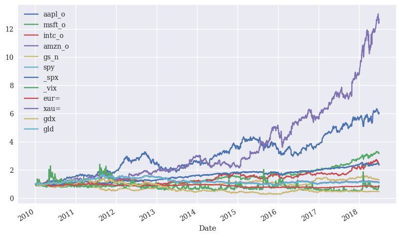
If you take the cumulative sum of log returns (R) at any point and do e^R, then you get the value of $1 invested at the beginning. We can use .apply() to “apply” the exponential function e to each value in the DataFrame. If you want to convert back to the cumulative simple return instead, you can do e^R - 1.
rets_log.cumsum().apply(np.exp)
| aapl_o | msft_o | intc_o | amzn_o | gs_n | spy | _spx | _vix | eur= | xau= | gdx | gld | |
|---|---|---|---|---|---|---|---|---|---|---|---|---|
| Date | ||||||||||||
| 2010-01-04 | NaN | NaN | NaN | NaN | NaN | NaN | NaN | NaN | NaN | NaN | NaN | NaN |
| 2010-01-05 | 1.001729 | 1.000323 | 0.999521 | 1.005900 | 1.017680 | 1.002647 | 1.003116 | 0.965569 | 0.997016 | 0.998795 | 1.009642 | 0.999089 |
| 2010-01-06 | 0.985795 | 0.994184 | 0.996169 | 0.987677 | 1.006818 | 1.003353 | 1.003663 | 0.956088 | 1.000069 | 1.016518 | 1.034165 | 1.015574 |
| 2010-01-07 | 0.983973 | 0.983910 | 0.986590 | 0.970874 | 1.026520 | 1.007588 | 1.007679 | 0.951098 | 0.993547 | 1.010625 | 1.029134 | 1.009290 |
| 2010-01-08 | 0.990514 | 0.990630 | 0.997605 | 0.997162 | 1.007107 | 1.010941 | 1.010583 | 0.904691 | 1.000069 | 1.014375 | 1.044645 | 1.014299 |
| ... | ... | ... | ... | ... | ... | ... | ... | ... | ... | ... | ... | ... |
| 2018-06-25 | 5.958559 | 3.178998 | 2.428640 | 12.420836 | 1.279986 | 2.391247 | 2.398141 | 0.864770 | 0.812019 | 1.129464 | 0.461329 | 1.091894 |
| 2018-06-26 | 6.032481 | 3.201292 | 2.378831 | 12.629500 | 1.280217 | 2.396541 | 2.403428 | 0.794411 | 0.808063 | 1.123786 | 0.460071 | 1.086157 |
| 2018-06-27 | 6.023650 | 3.151535 | 2.335249 | 12.401120 | 1.272128 | 2.376688 | 2.382748 | 0.893713 | 0.801610 | 1.117518 | 0.457137 | 1.079964 |
| 2018-06-28 | 6.067480 | 3.186753 | 2.358716 | 12.706871 | 1.290848 | 2.390276 | 2.397470 | 0.840818 | 0.802651 | 1.114179 | 0.459652 | 1.076685 |
| 2018-06-29 | 6.054723 | 3.186107 | 2.380747 | 12.694548 | 1.274382 | 2.393717 | 2.399289 | 0.802894 | 0.810700 | 1.118080 | 0.467617 | 1.080601 |
2138 rows × 12 columns
print(np.exp(1.800839))
6.054725248468137
You can then plot the cumulative returns. Notice how we use the . to keep sending the DataFrame through to the next step. Take the raw data, do something to it, do something else to that result, and then plot it.
rets_log.cumsum().apply(np.exp).plot(figsize=(10, 6));
We can also create return series using simple returns. We calculate percent returns, add 1 to each to get (1+R), and then chain returns together using .cumprod(). We subtract one at the end from the total.
In other words,
rets_simple = stocks.pct_change() # period return
rets_simple = rets_simple.add(1)
rets_simple.head()
| aapl_o | msft_o | intc_o | amzn_o | gs_n | spy | _spx | _vix | eur= | xau= | gdx | gld | |
|---|---|---|---|---|---|---|---|---|---|---|---|---|
| Date | ||||||||||||
| 2010-01-04 | NaN | NaN | NaN | NaN | NaN | NaN | NaN | NaN | NaN | NaN | NaN | NaN |
| 2010-01-05 | 1.001729 | 1.000323 | 0.999521 | 1.005900 | 1.017680 | 1.002647 | 1.003116 | 0.965569 | 0.997016 | 0.998795 | 1.009642 | 0.999089 |
| 2010-01-06 | 0.984094 | 0.993863 | 0.996646 | 0.981884 | 0.989327 | 1.000704 | 1.000546 | 0.990181 | 1.003062 | 1.017745 | 1.024289 | 1.016500 |
| 2010-01-07 | 0.998151 | 0.989665 | 0.990385 | 0.982987 | 1.019568 | 1.004221 | 1.004001 | 0.994781 | 0.993478 | 0.994203 | 0.995136 | 0.993812 |
| 2010-01-08 | 1.006648 | 1.006830 | 1.011165 | 1.027077 | 0.981089 | 1.003328 | 1.002882 | 0.951207 | 1.006565 | 1.003711 | 1.015071 | 1.004963 |
rets_simple_cumulative = rets_simple.cumprod().sub(1)
rets_simple_cumulative
| aapl_o | msft_o | intc_o | amzn_o | gs_n | spy | _spx | _vix | eur= | xau= | gdx | gld | |
|---|---|---|---|---|---|---|---|---|---|---|---|---|
| Date | ||||||||||||
| 2010-01-04 | NaN | NaN | NaN | NaN | NaN | NaN | NaN | NaN | NaN | NaN | NaN | NaN |
| 2010-01-05 | 0.001729 | 0.000323 | -0.000479 | 0.005900 | 0.017680 | 0.002647 | 0.003116 | -0.034431 | -0.002984 | -0.001205 | 0.009642 | -0.000911 |
| 2010-01-06 | -0.014205 | -0.005816 | -0.003831 | -0.012323 | 0.006818 | 0.003353 | 0.003663 | -0.043912 | 0.000069 | 0.016518 | 0.034165 | 0.015574 |
| 2010-01-07 | -0.016027 | -0.016090 | -0.013410 | -0.029126 | 0.026520 | 0.007588 | 0.007679 | -0.048902 | -0.006453 | 0.010625 | 0.029134 | 0.009290 |
| 2010-01-08 | -0.009486 | -0.009370 | -0.002395 | -0.002838 | 0.007107 | 0.010941 | 0.010583 | -0.095309 | 0.000069 | 0.014375 | 0.044645 | 0.014299 |
| ... | ... | ... | ... | ... | ... | ... | ... | ... | ... | ... | ... | ... |
| 2018-06-25 | 4.958559 | 2.178998 | 1.428640 | 11.420836 | 0.279986 | 1.391247 | 1.398141 | -0.135230 | -0.187981 | 0.129464 | -0.538671 | 0.091894 |
| 2018-06-26 | 5.032481 | 2.201292 | 1.378831 | 11.629500 | 0.280217 | 1.396541 | 1.403428 | -0.205589 | -0.191937 | 0.123786 | -0.539929 | 0.086157 |
| 2018-06-27 | 5.023650 | 2.151535 | 1.335249 | 11.401120 | 0.272128 | 1.376688 | 1.382748 | -0.106287 | -0.198390 | 0.117518 | -0.542863 | 0.079964 |
| 2018-06-28 | 5.067480 | 2.186753 | 1.358716 | 11.706871 | 0.290848 | 1.390276 | 1.397470 | -0.159182 | -0.197349 | 0.114179 | -0.540348 | 0.076685 |
| 2018-06-29 | 5.054723 | 2.186107 | 1.380747 | 11.694548 | 0.274382 | 1.393717 | 1.399289 | -0.197106 | -0.189300 | 0.118080 | -0.532383 | 0.080601 |
2138 rows × 12 columns
Normalizing price series#
You often see charts where all of the assets start at a price of 1 or 100. You can then compare their growth over time. We can easily do this using pandas.
We can divide all of the prices by the first price in the series, creating prices relative to that starting point.
We can pull the first price for one stock using .iloc.
stocks.aapl_o.iloc[0]
30.57282657
We can also pull all of the first prices.
stocks.iloc[0]
aapl_o      30.572827
msft_o      30.950000
intc_o      20.880000
amzn_o     133.900000
gs_n       173.080000
spy        113.330000
_spx      1132.990000
_vix        20.040000
eur=         1.441100
xau=      1120.000000
gdx         47.710000
gld        109.800000
Name: 2010-01-04 00:00:00, dtype: float64
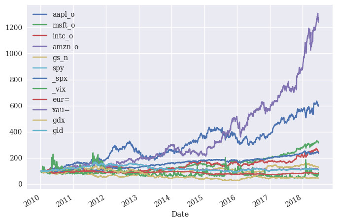
We can use .div() to divide every item in a column by the first item in that column. This is yet another example of vectorization making our lives easier. As the DataCamp assignment notes, .div() and other math functions automatically align series and DataFrame columns. So, each price in the first column gets divided by the first price in the first column, etc.
normalized = stocks.div(stocks.iloc[0]).mul(100)
normalized.plot()
<Axes: xlabel='Date'>
Resampling#
Resampling is when you change the time period that you’re looking at. So, you can go from daily to weekly to monthly, etc. This is called downsampling and involves aggregating your data.
Resampling allows us to aggregate data at different time intervals and even perform calculations as we go. For example, we can convert daily data into monthly averages using:
monthly_data = df.resample("M").mean() # Aggregates data by month
This works by:
Grouping data by end-of-month dates.
Taking the mean of all daily values in that month.
Creating a new DataFrame with monthly frequency.
You can also do the opposite and go from, say, monthly to daily. The new dates created in your data will be set as NaN. This is called upsampling and involves filling in missing data.
How is .resample() different from .groupby()?
.resample("M")creates a new index with ALL months, even if some months have missing data..groupby(df.index.month).mean()groups only existing months (missing months are NOT included).
Let’s start with .asfreq and some basic fill methods. I am going to “create” some quarterly data first for us to work with. I’ll discuss how I do this in a minute.
.asfreq() is a method that allows us to change the frequency of our time series data. We can use it to upsample or downsample our data.
You should also check for missing values before you start resampling. You can use .isnull().sum() to see how many missing values you have.
stocks_quarterly = stocks.resample('1QE', label='right').last()
stocks_quarterly.head()
| aapl_o | msft_o | intc_o | amzn_o | gs_n | spy | _spx | _vix | eur= | xau= | gdx | gld | |
|---|---|---|---|---|---|---|---|---|---|---|---|---|
| Date | ||||||||||||
| 2010-03-31 | 33.571395 | 29.2875 | 22.29 | 135.77 | 170.63 | 117.00 | 1169.43 | 17.59 | 1.3510 | 1112.80 | 44.41 | 108.95 |
| 2010-06-30 | 35.932821 | 23.0100 | 19.45 | 109.26 | 131.27 | 103.22 | 1030.71 | 34.54 | 1.2234 | 1241.35 | 51.96 | 121.68 |
| 2010-09-30 | 40.535674 | 24.4900 | 19.20 | 157.06 | 144.58 | 114.13 | 1141.20 | 23.70 | 1.3630 | 1308.50 | 55.93 | 127.91 |
| 2010-12-31 | 46.079954 | 27.9100 | 21.03 | 180.00 | 168.16 | 125.75 | 1257.64 | 17.75 | 1.3377 | 1419.45 | 61.47 | 138.72 |
| 2011-03-31 | 49.786736 | 25.3900 | 20.18 | 180.13 | 158.47 | 132.59 | 1325.83 | 17.74 | 1.4165 | 1430.00 | 60.10 | 139.86 |
Alright, we have some quarterly stock price data now. But, what if I want to make this monthly data? Well, I don’t have the actual monthly prices in this data set, but I can still upsample the data and go from quarterly to monthly.
stocks_monthly = stocks_quarterly.asfreq('ME')
stocks_monthly.head()
| aapl_o | msft_o | intc_o | amzn_o | gs_n | spy | _spx | _vix | eur= | xau= | gdx | gld | |
|---|---|---|---|---|---|---|---|---|---|---|---|---|
| Date | ||||||||||||
| 2010-03-31 | 33.571395 | 29.2875 | 22.29 | 135.77 | 170.63 | 117.00 | 1169.43 | 17.59 | 1.3510 | 1112.80 | 44.41 | 108.95 |
| 2010-04-30 | NaN | NaN | NaN | NaN | NaN | NaN | NaN | NaN | NaN | NaN | NaN | NaN |
| 2010-05-31 | NaN | NaN | NaN | NaN | NaN | NaN | NaN | NaN | NaN | NaN | NaN | NaN |
| 2010-06-30 | 35.932821 | 23.0100 | 19.45 | 109.26 | 131.27 | 103.22 | 1030.71 | 34.54 | 1.2234 | 1241.35 | 51.96 | 121.68 |
| 2010-07-31 | NaN | NaN | NaN | NaN | NaN | NaN | NaN | NaN | NaN | NaN | NaN | NaN |
We now have new dates and missing values. This is expected, though. We’ve created new observations out of new dates. We could fill in these missing values like we want. .asfreq() has different methods. I’ll fill with the previous value, so that April and May get a March value, etc. This is called a forward fill.
stocks_monthly = stocks_quarterly.asfreq('ME').ffill()
stocks_monthly.head()
| aapl_o | msft_o | intc_o | amzn_o | gs_n | spy | _spx | _vix | eur= | xau= | gdx | gld | |
|---|---|---|---|---|---|---|---|---|---|---|---|---|
| Date | ||||||||||||
| 2010-03-31 | 33.571395 | 29.2875 | 22.29 | 135.77 | 170.63 | 117.00 | 1169.43 | 17.59 | 1.3510 | 1112.80 | 44.41 | 108.95 |
| 2010-04-30 | 33.571395 | 29.2875 | 22.29 | 135.77 | 170.63 | 117.00 | 1169.43 | 17.59 | 1.3510 | 1112.80 | 44.41 | 108.95 |
| 2010-05-31 | 33.571395 | 29.2875 | 22.29 | 135.77 | 170.63 | 117.00 | 1169.43 | 17.59 | 1.3510 | 1112.80 | 44.41 | 108.95 |
| 2010-06-30 | 35.932821 | 23.0100 | 19.45 | 109.26 | 131.27 | 103.22 | 1030.71 | 34.54 | 1.2234 | 1241.35 | 51.96 | 121.68 |
| 2010-07-31 | 35.932821 | 23.0100 | 19.45 | 109.26 | 131.27 | 103.22 | 1030.71 | 34.54 | 1.2234 | 1241.35 | 51.96 | 121.68 |
pandas also has a method called .resample. This is a lot like a .groupby(), but dealing with time.
The code stocks.resample('1w', label='right') creates what pandas calls a DatetimeIndexResampler object. Basically, we are creating “bins” based on the time period we specify. I start with one week and then do one month. The argument label='right' tells .resample() which bin edge to label the bucket with. So, the first edge (i.e. the first date)
or the last edge (i.e. the last date). The option right means the last edge. For example, the bin will get labeled with the last day of the week. Or the last day of the month. The method .last() picks the last member of each time bin. So, we’ll get get end-of-week prices or end-of-month prices.
You can find the documentation here.
stocks.resample('1W', label='right').last().head()
| aapl_o | msft_o | intc_o | amzn_o | gs_n | spy | _spx | _vix | eur= | xau= | gdx | gld | |
|---|---|---|---|---|---|---|---|---|---|---|---|---|
| Date | ||||||||||||
| 2010-01-10 | 30.282827 | 30.66 | 20.83 | 133.52 | 174.31 | 114.57 | 1144.98 | 18.13 | 1.4412 | 1136.10 | 49.84 | 111.37 |
| 2010-01-17 | 29.418542 | 30.86 | 20.80 | 127.14 | 165.21 | 113.64 | 1136.03 | 17.91 | 1.4382 | 1129.90 | 47.42 | 110.86 |
| 2010-01-24 | 28.249972 | 28.96 | 19.91 | 121.43 | 154.12 | 109.21 | 1091.76 | 27.31 | 1.4137 | 1092.60 | 43.79 | 107.17 |
| 2010-01-31 | 27.437544 | 28.18 | 19.40 | 125.41 | 148.72 | 107.39 | 1073.87 | 24.62 | 1.3862 | 1081.05 | 40.72 | 105.96 |
| 2010-02-07 | 27.922829 | 28.02 | 19.47 | 117.39 | 154.16 | 106.66 | 1066.19 | 26.11 | 1.3662 | 1064.95 | 42.41 | 104.68 |
stocks.resample('1ME', label='right').last().head()
| aapl_o | msft_o | intc_o | amzn_o | gs_n | spy | _spx | _vix | eur= | xau= | gdx | gld | |
|---|---|---|---|---|---|---|---|---|---|---|---|---|
| Date | ||||||||||||
| 2010-01-31 | 27.437544 | 28.1800 | 19.40 | 125.41 | 148.72 | 107.3900 | 1073.87 | 24.62 | 1.3862 | 1081.05 | 40.72 | 105.960 |
| 2010-02-28 | 29.231399 | 28.6700 | 20.53 | 118.40 | 156.35 | 110.7400 | 1104.49 | 19.50 | 1.3625 | 1116.10 | 43.89 | 109.430 |
| 2010-03-31 | 33.571395 | 29.2875 | 22.29 | 135.77 | 170.63 | 117.0000 | 1169.43 | 17.59 | 1.3510 | 1112.80 | 44.41 | 108.950 |
| 2010-04-30 | 37.298534 | 30.5350 | 22.84 | 137.10 | 145.20 | 118.8125 | 1186.69 | 22.05 | 1.3295 | 1178.25 | 50.51 | 115.360 |
| 2010-05-31 | 36.697106 | 25.8000 | 21.42 | 125.46 | 144.26 | 109.3690 | 1089.41 | 32.07 | 1.2267 | 1213.81 | 49.86 | 118.881 |
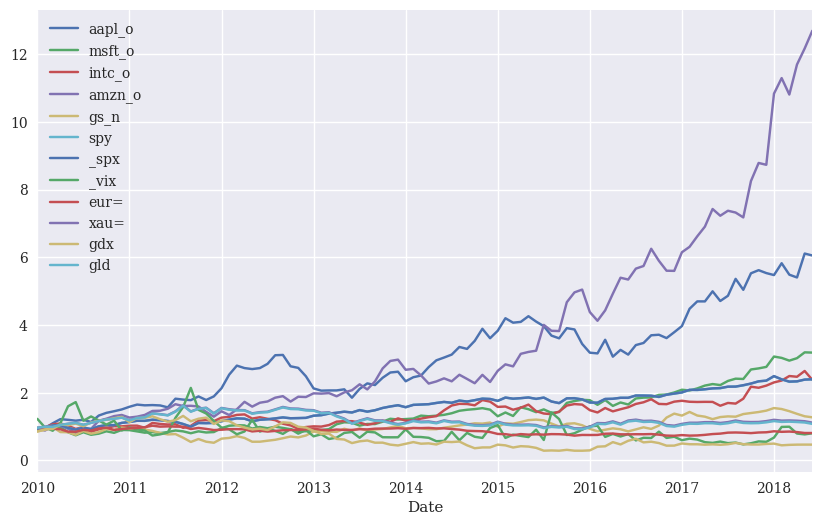
rets_log.cumsum().apply(np.exp).resample('1ME', label='right').last(
                          ).plot(figsize=(10, 6));
Rolling statistics#
Rolling statistics are your usual sorts of statistics, like a mean or standard deviation, but calculated with rolling time windows. So, the average price over the past month. Or, the standard deviation of returns of the past year. The value gets updated as you move forward in time - this is the rolling part.
Let’s set a 20 day window and calculate some rolling statistics. There’s one you might not know, a kind of moving average called an exponentially weighted moving average (ewma).
window = 20

stocks['aapl_min'] = stocks['aapl_o'].rolling(window=window).min()
stocks['aapl_mean'] = stocks['aapl_o'].rolling(window=window).mean()
stocks['aapl_std'] = stocks['aapl_o'].rolling(window=window).std()
stocks['aapl_max'] = stocks['aapl_o'].rolling(window=window).max()
stocks['aapl_ewma'] = stocks['aapl_o'].ewm(halflife=0.5, min_periods=window).mean()
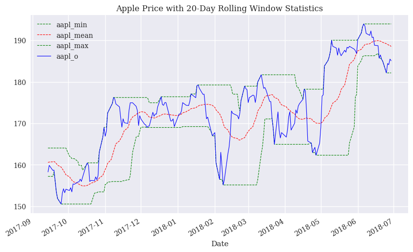
Let’s make a plot using pandas plot. I’ll select four variables and then pick just the last 200 observations using .iloc. Notice I don’t need to include the index value. This is a line graph, so .plot() knows that you want this on the x-axis. I like how .plot() automatically styles the x-axis for us too.
stocks[['aapl_min', 'aapl_mean', 'aapl_max', 'aapl_o']].iloc[-200:].plot(style=['g--', 'r--', 'g--', 'b'], lw=0.8, figsize=(10, 6), title = 'Apple Price with 20-Day Rolling Window Statistics');
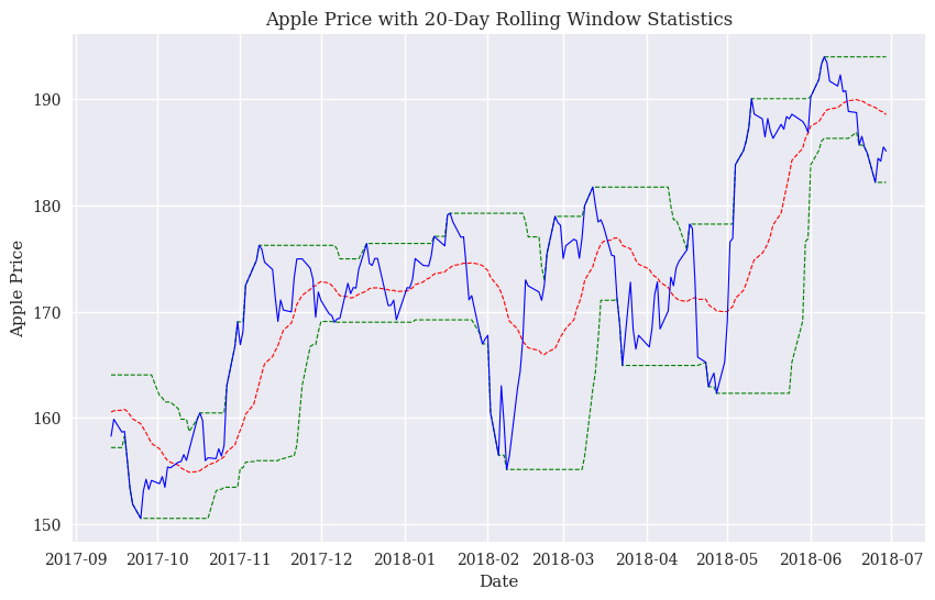
Now, I’ll make the same graph using matplotlib. Again, I don’t include the index value, as, by default, matplotlib will put it on the x-axis. I’m going to put four different line plots on the same axis. I am again selecting just the last 200 rows using .iloc().
fig = plt.figure(figsize=(10, 6))

ax = fig.add_subplot(1, 1, 1)

ax.plot(stocks.aapl_min.iloc[-200:], 'g--', lw=0.8)
ax.plot(stocks.aapl_mean.iloc[-200:], 'r--', lw=0.8)
ax.plot(stocks.aapl_max.iloc[-200:], 'g--', lw=0.8)
ax.plot(stocks.aapl_o.iloc[-200:], 'b', lw=0.8)

ax.set_xlabel('Date')
ax.set_ylabel('Apple Price')
ax.set_title('Apple Price with 20-Day Rolling Window Statistics');
Which way should you make your plots? Basically up to you! There are less verbose ways to do it that the matplotlib method I used above. I kind of like seeing each line like that, as it helps me read and understand what’s going on.
You could also select just the data you want, save it to a new DataFrame, and then plot.
stocks_last200 = stocks.iloc[-200:]

fig = plt.figure(figsize=(10, 6))

ax = fig.add_subplot(1, 1, 1)

ax.plot(stocks_last200.aapl_min, 'g--', lw=0.8)
ax.plot(stocks_last200.aapl_mean, 'r--', lw=0.8)
ax.plot(stocks_last200.aapl_max, 'g--', lw=0.8)
ax.plot(stocks_last200.aapl_o, 'b', lw=0.8)

ax.set_xlabel('Date')
ax.set_ylabel('Apple Price')
ax.set_title('Apple Price with 20-Day Rolling Window Statistics');
Simple trend indicator#
One of the best known “anomalies” in finance is that stocks that have been doing better perform better in the future, and vice-versa. This general set of anomalies are called momentum and trend. Here’s a summary of momentum and why it might exist. The hedge fund Two Sigma has a brief explanation of how trend and momentum are different. And a more academic explanation.
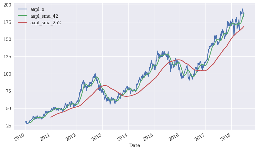
We can calculate basic moving averages that might capture the spirit of trend. We want stocks that are outperforming their longer history in the short-term. We can measure this with two different simple moving averages (sma).
stocks['aapl_sma_42'] = stocks['aapl_o'].rolling(window=42).mean()
stocks['aapl_sma_252'] = stocks['aapl_o'].rolling(window=252).mean()

stocks[['aapl_o', 'aapl_sma_42', 'aapl_sma_252']].plot(figsize=(10, 6));
Let’s create an indicator (1/0) variable that is 1 if the two-month moving average is above the one-year moving average. This would be example of a simple short-term trend strategy. You buy the stock if it is doing better now than it has in over the past year. You do not own the stock otherwise.
I will then graph the moving averages, the price, and the indicator, called take_position, on the same graph. I’m going to do something a bit different, but you’ll see it in our text. I will use pandas .plot() to make the graph, but save this to an axes object. I can then refer to the ax object when styling. This kind of mixes two ways that we’ve seen plot and figure creation!
Notice the creation of a secondary y-axis for the indicator variable.
stocks['take_position'] = np.where(stocks['aapl_sma_42'] > stocks['aapl_sma_252'], 1, -1)

ax = stocks[['aapl_o', 'aapl_sma_42', 'aapl_sma_252', 'take_position']].plot(figsize=(10, 6), secondary_y='take_position')
ax.get_legend().set_bbox_to_anchor((0.25, 0.85));
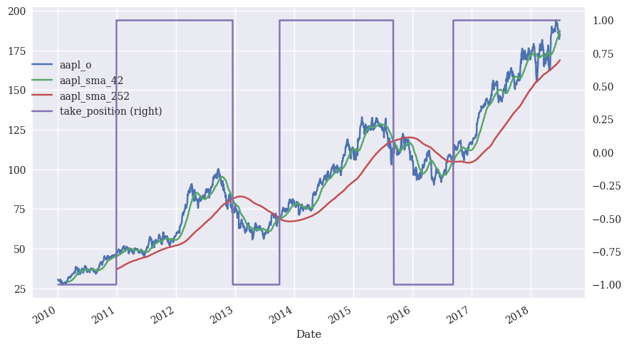
What do you think? Did this strategy work for trading Apple during the 2010s? We’ll look more at backtesting strategies and all of the issues that arise later on.
Correlation and regression#
We’ll look at some simple correlation and linear regression calculations. We’ll do more with regression later on.
Let’s look at the relationship between the S&P 500 and the Apple. I’ll bring the stocks data again, but just keep these two time series. I won’t bother cleaning the names. pyjanitor replaces the . in front of .SPX with an underscore and plot() doesn’t like that when making the legend.
# Read in some eod prices
stocks2 = pd.read_csv('https://raw.githubusercontent.com/aaiken1/fin-data-analysis-python/main/data/tr_eikon_eod_data.csv',
index_col=0, parse_dates=True)
stocks2 = stocks2.dropna()
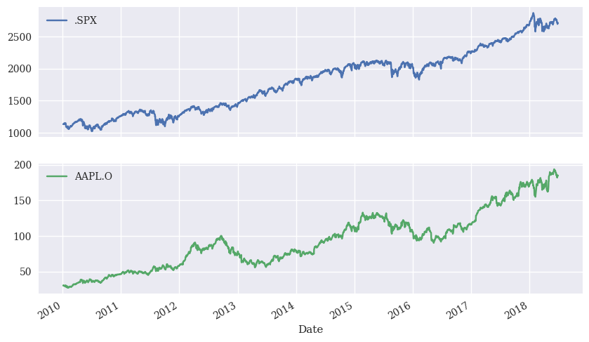
stocks2 = stocks2[['.SPX', 'AAPL.O']]
stocks2.plot(subplots=True, figsize=(10, 6));
rets2 = np.log(stocks2 / stocks2.shift(1))

rets2 = rets2.dropna()
pd.plotting.scatter_matrix(rets2,
                           alpha=0.2,
                           diagonal='hist',
                           hist_kwds={'bins': 35},
                           figsize=(10, 6));

rets2
| .SPX | AAPL.O | |
|---|---|---|
| Date | ||
| 2010-01-05 | 0.003111 | 0.001727 |
| 2010-01-06 | 0.000545 | -0.016034 |
| 2010-01-07 | 0.003993 | -0.001850 |
| 2010-01-08 | 0.002878 | 0.006626 |
| 2010-01-11 | 0.001745 | -0.008861 |
| ... | ... | ... |
| 2018-06-25 | -0.013820 | -0.014983 |
| 2018-06-26 | 0.002202 | 0.012330 |
| 2018-06-27 | -0.008642 | -0.001465 |
| 2018-06-28 | 0.006160 | 0.007250 |
| 2018-06-29 | 0.000758 | -0.002105 |
2137 rows × 2 columns
Yikes! Not sure about those y-axis labels. That’s some floating-point nonsense.
We can run a simple linear regression using np.polyfit from the numpy library. Other libraries have more sophisticated tools. We’ll set deg=1 since this is a linear regression (i.e. degree of 1).
reg = np.polyfit(rets2['.SPX'], rets2['AAPL.O'], deg=1)
reg
array([9.57422130e-01, 4.50598662e-04])
Apple has a beta of 0.957 (note the scientific notation in the output). The intercept (or alpha) is the next number and is based on daily returns.
rets2.corr()
| .SPX | AAPL.O | |
|---|---|---|
| .SPX | 1.000000 | 0.563036 |
| AAPL.O | 0.563036 | 1.000000 |
Generating random returns#
We are going to look more at distributions and what are called Monte Carlo methods when we get to risk management, simulations, and option pricing. But, for now, let’s look at a simple case of generating some random returns that “look” like actual stock returns.
Let’s create 1000 random numbers from a normal distribution with a mean of 0 and a standard deviation of 0.01 (1%). This means that we “pull” these numbers out of that distribution. We can then plot them (using seaborn, for fun) and include a normal distribution that fits the distribution of random numbers.
seed(1986)
random_returns = normal(loc=0, scale=0.01, size=1000)

# Plot histogram with a fitted normal distribution overlay
fig, ax = plt.subplots(figsize=(8, 5))
sns.histplot(random_returns, stat='density', kde=False, ax=ax)

# Overlay the normal distribution curve
x = np.linspace(random_returns.min(), random_returns.max(), 100)
ax.plot(x, norm.pdf(x, loc=random_returns.mean(), scale=random_returns.std()), 'r-', lw=2, label='Normal fit')
ax.legend()
ax.set_title('Simulated Random Returns')
ax.set_xlabel('Return');
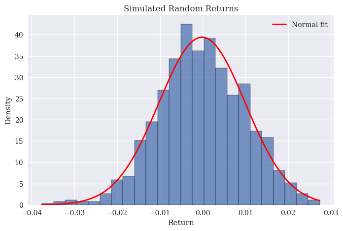
Looks like a bell curve to me. Let’s take that set of 1000 random numbers and turn them into a pd.Series. We can then treat them like actual returns and create a cumulative return series, like above.
return_series = pd.Series(random_returns)
random_prices = return_series.add(1).cumprod().sub(1)
random_prices.mul(100).plot();
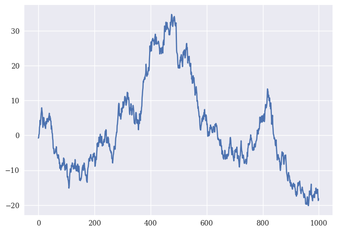
And there you go! Some fake returns. Stocks returns aren’t actually normally distributed like this, at least over short windows. Simulations and Monte Carlo methods are used a lot in wealth management to figure out the probability that a client will meet their retirement goals.
The distribution of real returns#
We just generated random returns from a normal distribution. They looked like a nice bell curve. But do real stock returns actually follow a normal distribution? This turns out to be one of the most important questions in finance, because so many models – from portfolio optimization to option pricing – assume that they do.
The material in this section draws on ideas from Professor Jonathan Hersh’s course on Generative AI in Finance at Chapman University (Spring 2026).
The normal distribution assumption#
The normal distribution (the Gaussian bell curve) underpins most classical finance models. If returns are normally distributed, then:
Returns are symmetric around the mean
68% of observations fall within 1 standard deviation of the mean
95% fall within 2 standard deviations
99.7% fall within 3 standard deviations
Under these assumptions, extreme events – returns beyond 3 standard deviations from the mean – should be extraordinarily rare. A “6-sigma event” should occur roughly once every 4 million trading days, or about once every 16,000 years.
But look at what happens when we overlay actual S&P 500 daily returns against a normal distribution with the same mean and standard deviation:
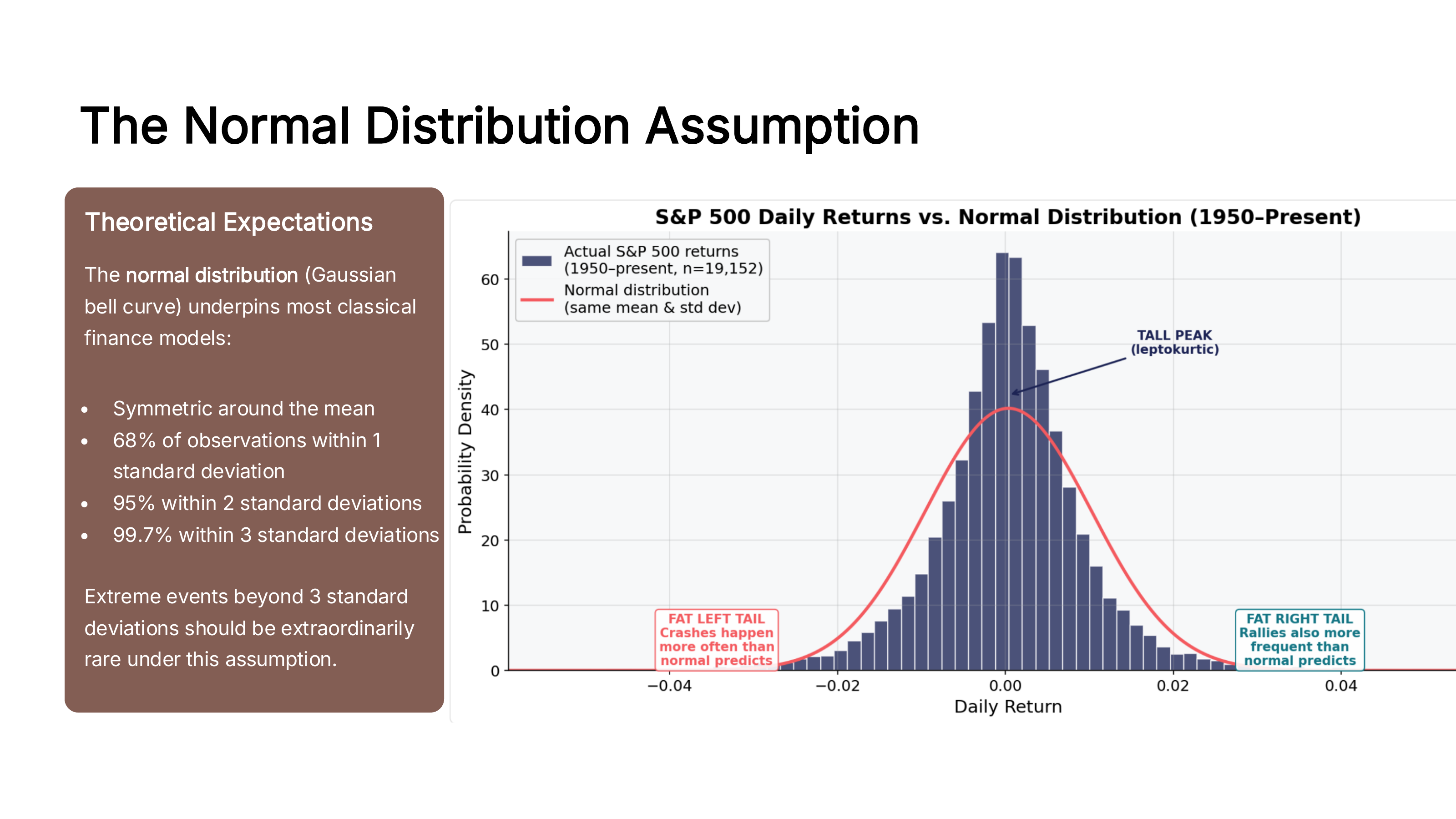
Fig. 47 Actual S&P 500 daily returns (1950-present) overlaid with a normal distribution. Notice the taller peak in the center and the fatter tails on both sides. Source: Professor Jonathan Hersh, BUS 696: Generative AI in Finance, Chapman University, Spring 2026.#
The actual distribution has a taller peak (more “normal” days clustered near zero) and fatter tails (more extreme days than the bell curve predicts). This pattern is called leptokurtic – it’s the same concept of kurtosis we discuss in the portfolio math chapter.
Fat tails: the reality#
The difference becomes dramatic when you zoom in on the tails. The chart below compares actual S&P 500 returns against both a normal distribution and a Student’s t-distribution (which has heavier tails). The right panel uses a log scale on the y-axis, which makes the tails easier to see. The normal distribution underestimates the probability of extreme events by 10-100x.
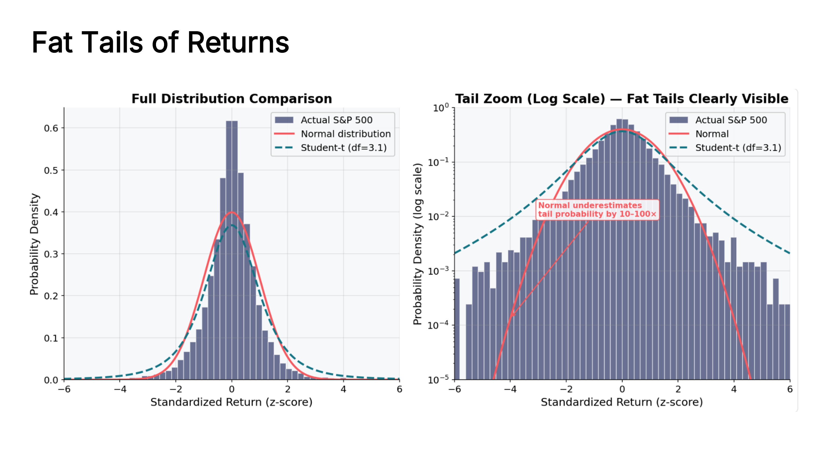
Fig. 48 Full distribution comparison (left) and tail zoom on a log scale (right). The normal distribution (red) dramatically underestimates tail probabilities compared to actual S&P 500 returns. The Student’s t-distribution (dashed teal) provides a much better fit. Source: Professor Jonathan Hersh, BUS 696: Generative AI in Finance, Chapman University, Spring 2026.#
How bad is this underestimation? The chart below compares what the normal distribution predicts for extreme events against what actually occurred in S&P 500 data since 1950. Beyond 4 standard deviations, reality outnumbers the prediction by roughly 91 times. Beyond 5 sigma, the normal distribution expects essentially zero events – but the S&P 500 has experienced dozens.
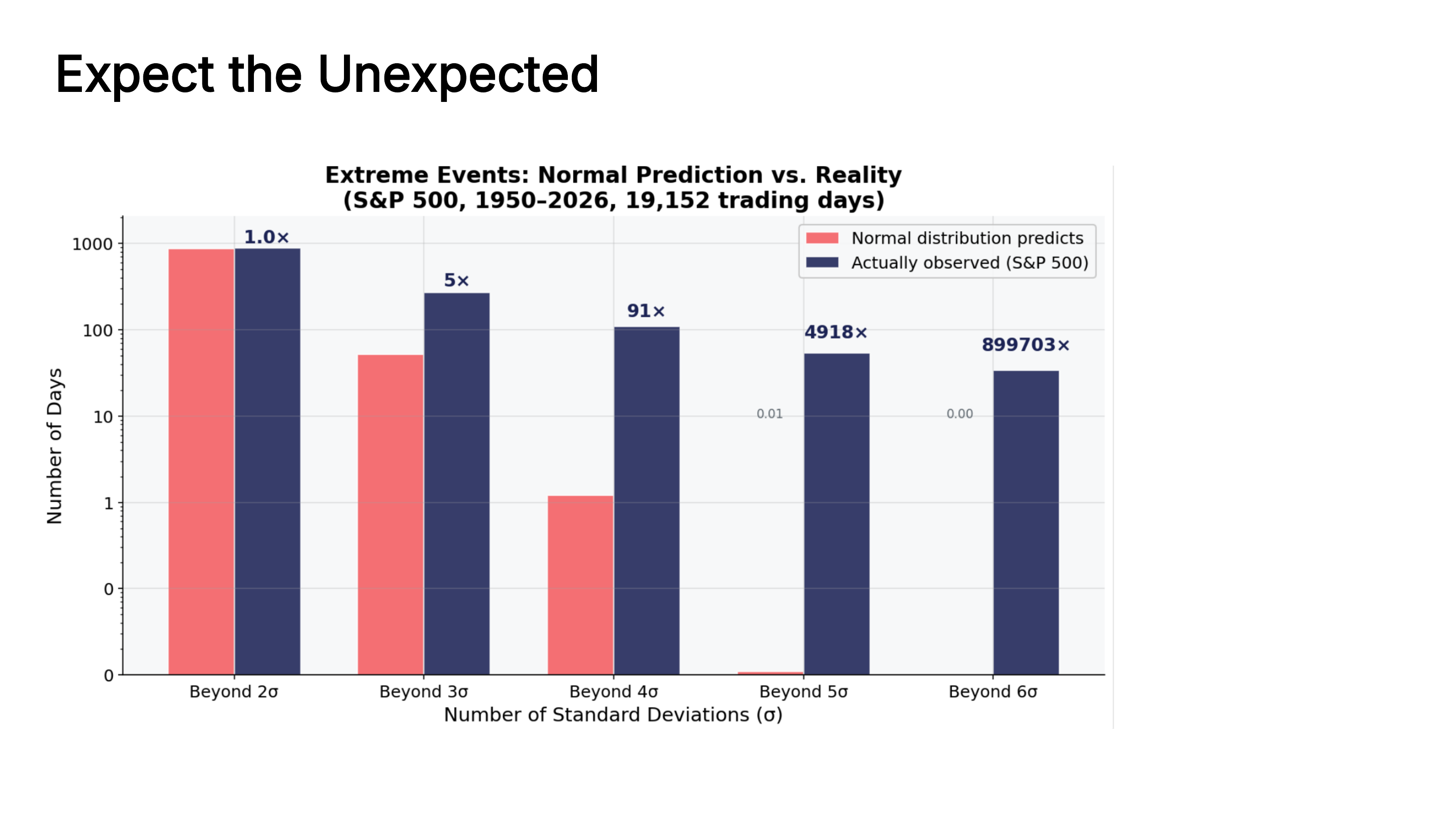
Fig. 49 Extreme events: what the normal distribution predicts vs. what actually happens. The multipliers (5x, 91x, 4918x, 899703x) show how severely the normal distribution underestimates tail risk at each sigma level. Source: Professor Jonathan Hersh, BUS 696: Generative AI in Finance, Chapman University, Spring 2026.#
These aren’t abstract statistical curiosities. Every entry on the timeline below is a real market crash that “shouldn’t have happened” under normal distribution assumptions. Black Monday (1987) was a 22-sigma event. The 2008 financial crisis registered as roughly a 25-sigma event – a probability so small it should essentially never occur in the lifetime of the universe, yet it happened.
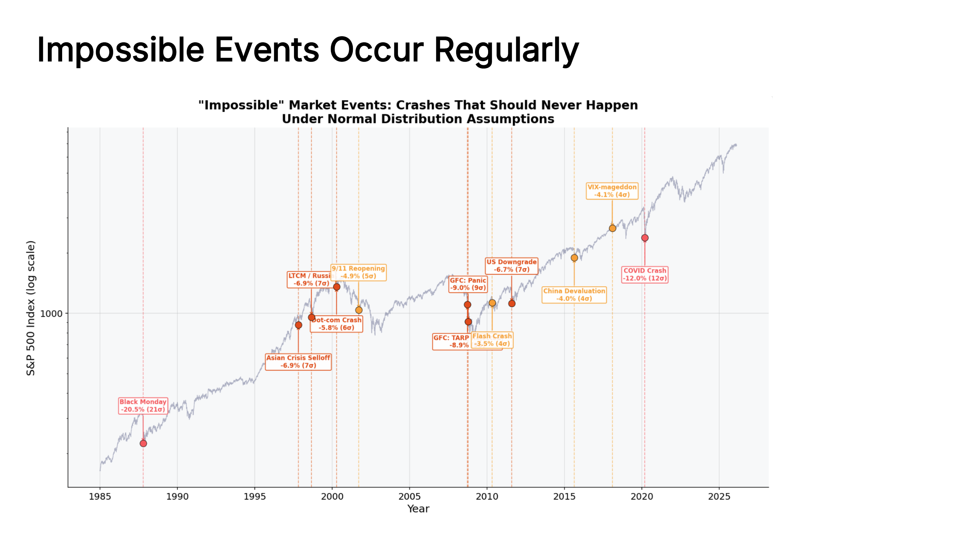
Fig. 50 A timeline of “impossible” market events – crashes that should never have happened under normal distribution assumptions. Each label shows the daily decline and the number of standard deviations. Source: Professor Jonathan Hersh, BUS 696: Generative AI in Finance, Chapman University, Spring 2026.#
Important
Fat tails mean that extreme market events – both crashes and rallies – happen far more often than standard models predict. This has enormous practical consequences for risk management, portfolio construction, and the pricing of options and other derivatives. We’ll come back to this idea in the risk management and Monte Carlo chapters.
Volatility clustering#
There’s another important feature of real financial returns: volatility clusters. Large moves (positive or negative) tend to be followed by more large moves, and calm periods tend to be followed by more calm periods. Volatility is not constant – it comes in bursts.
The chart below shows S&P 500 daily returns on top and rolling 21-day (one month) annualized volatility on the bottom. Notice how the spikes in volatility are concentrated during the 2008 financial crisis, the COVID crash in 2020, and the 2022 bear market. Between those crises, markets were relatively calm.
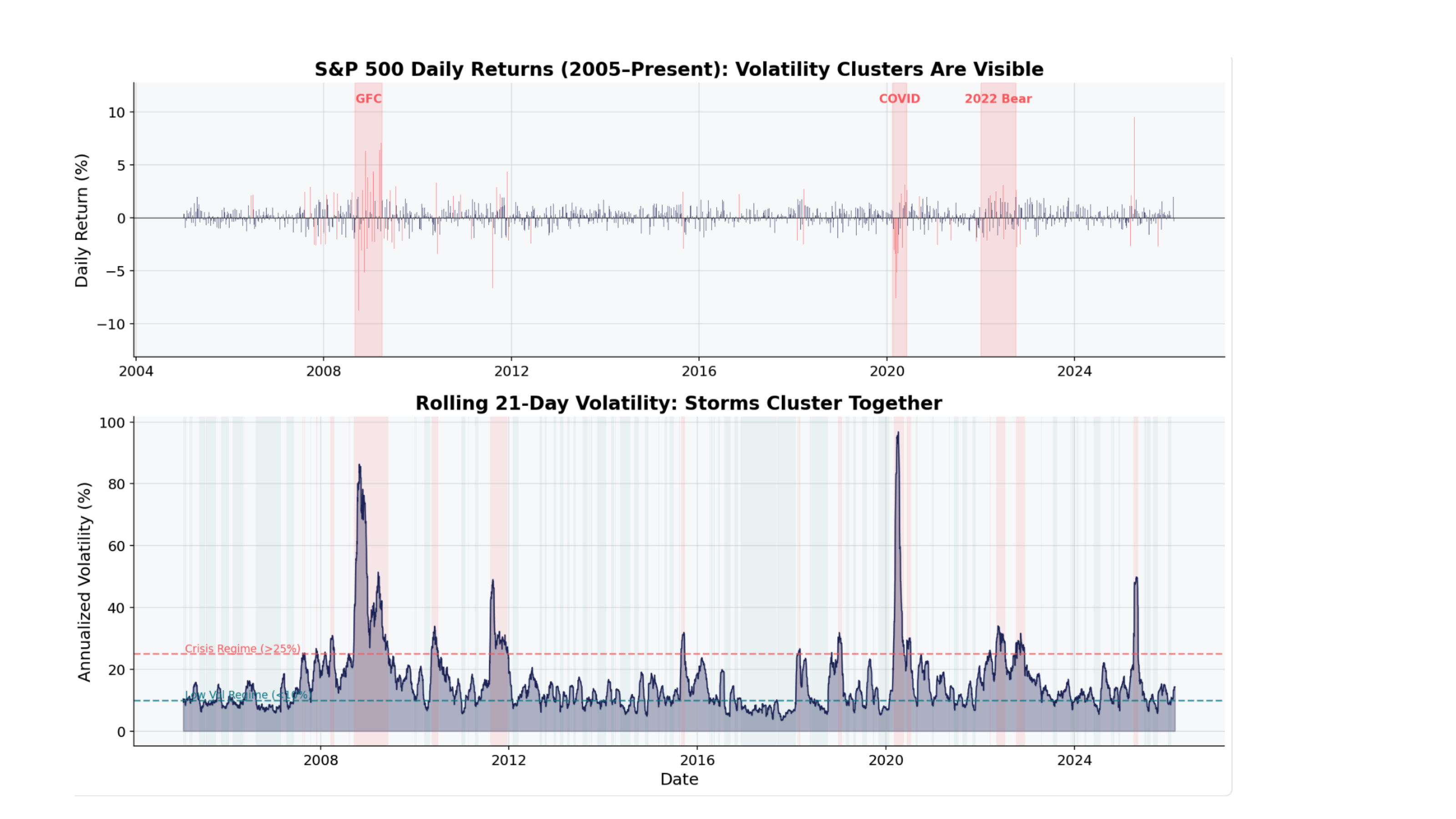
Fig. 51 S&P 500 daily returns (top) and rolling 21-day annualized volatility (bottom). Volatility comes in clusters – storms travel together. Source: Professor Jonathan Hersh, BUS 696: Generative AI in Finance, Chapman University, Spring 2026.#
This clustering behavior violates another assumption of simple models: that each day’s return is independent of the previous day’s return. In reality, knowing that today was a high-volatility day tells you that tomorrow is more likely to be high-volatility too. Financial econometricians model this with tools like GARCH (Generalized Autoregressive Conditional Heteroskedasticity) models, which allow volatility to change over time in a structured way.
Simple returns vs. log returns revisited#
We’ve already calculated both simple and log returns earlier in this chapter. But it’s worth revisiting why we have both, now that we’ve seen what real return distributions look like.
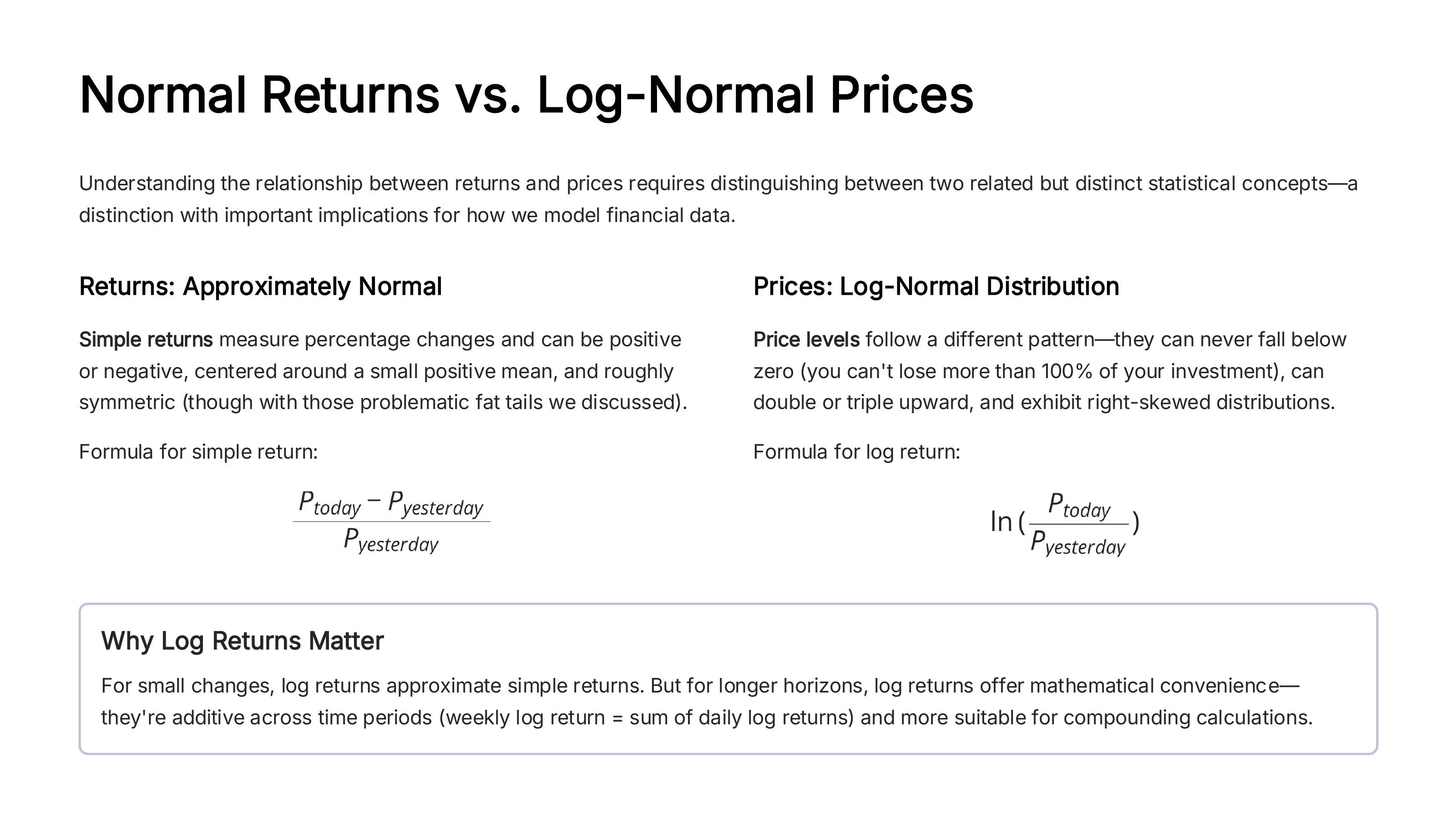
Fig. 52 Simple returns are approximately normal; prices follow a log-normal distribution. Log returns are additive over time, which makes them mathematically convenient. Source: Professor Jonathan Hersh, BUS 696: Generative AI in Finance, Chapman University, Spring 2026.#
Simple (discrete) returns measure the percentage change in price: \((P_{today} - P_{yesterday}) / P_{yesterday}\). They can be positive or negative, are centered around a small positive mean, and are roughly symmetric. We use these for portfolio optimization because the portfolio return is the weighted average of individual simple returns.
Log returns are the natural log of the price ratio: \(\ln(P_{today} / P_{yesterday})\). They have a key mathematical property: they are additive over time. A weekly log return equals the sum of the five daily log returns. This makes them convenient for cumulative return calculations and for statistical modeling.
For small returns (a few percent), the two are nearly identical. The difference grows for larger returns and over longer horizons.
Note
Here’s a practical rule of thumb: use simple returns when you need to combine returns across assets (portfolio math). Use log returns when you need to combine returns across time (cumulative returns, time series analysis). We used this property earlier when we computed rets_log.cumsum() to get cumulative returns.
Why this matters#
If returns were truly normally distributed, finance would be much simpler. Risk management would be straightforward – just multiply standard deviations. Market crashes would be virtually impossible. Value-at-Risk models would accurately predict losses.
But that’s not the world we live in.
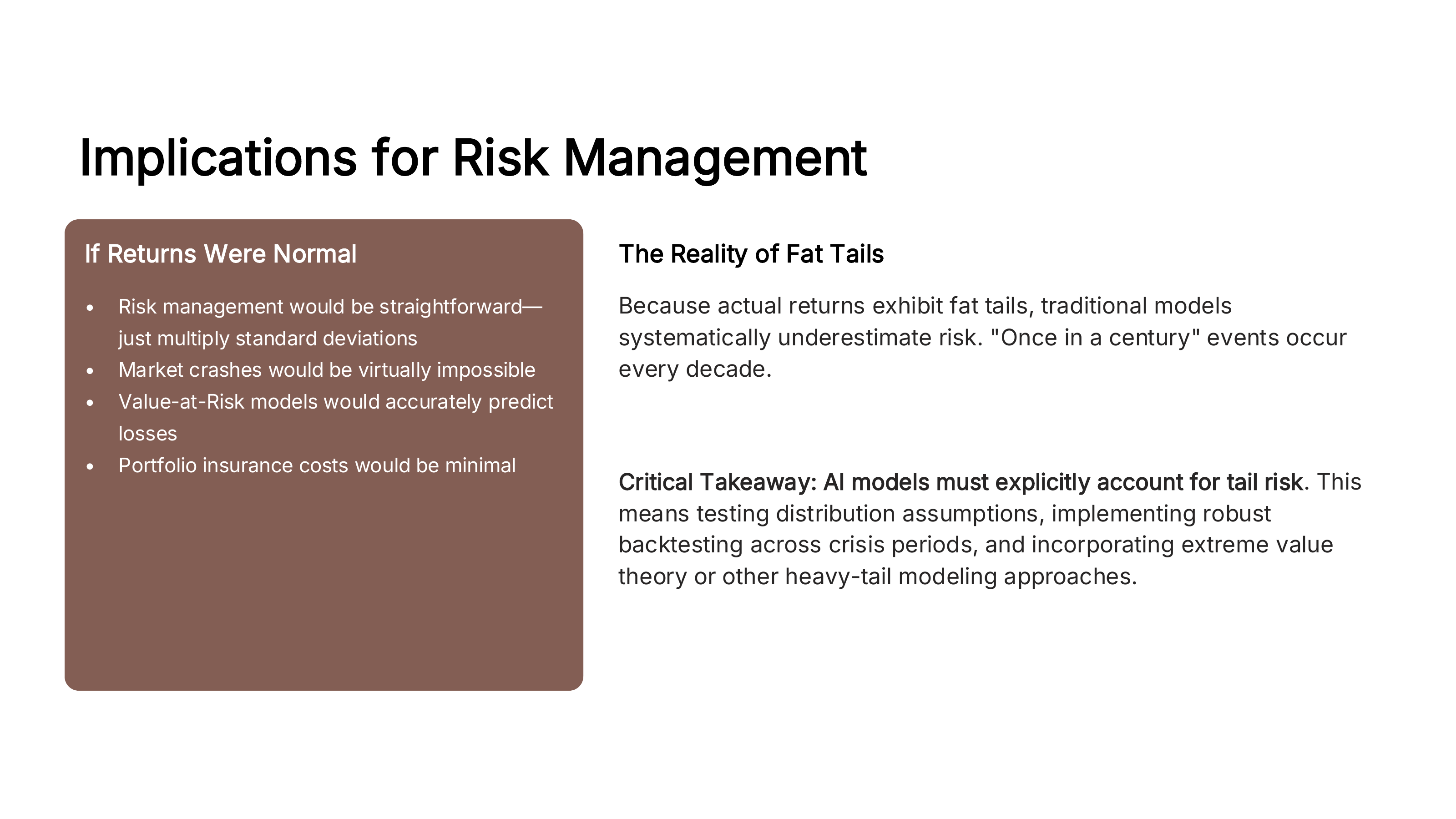
Fig. 53 The implications of fat tails for risk management. Traditional models systematically underestimate risk. Source: Professor Jonathan Hersh, BUS 696: Generative AI in Finance, Chapman University, Spring 2026.#
Because actual returns exhibit fat tails, traditional models systematically underestimate risk. “Once in a century” events seem to occur every decade. Any model or strategy that assumes normality – and many do, at least implicitly – will be caught off guard by the frequency of extreme events.
Important
Three key facts about real financial return distributions:
Fat tails: Extreme events happen far more often than the normal distribution predicts.
Volatility clustering: Calm periods and turbulent periods tend to persist. Volatility is not constant.
Slight negative skewness: Large negative returns (crashes) are somewhat more frequent than large positive returns (rallies) of the same magnitude.
Keep these in mind as we build models throughout the rest of the course. We’ll revisit distribution assumptions in the risk management and Monte Carlo simulation chapters.