
Portfolio optimization#
Portfolio optimization is an important part of many quantitative strategies. You take some inputs related to risk and return and you try to find the portfolio with the desired characteristics. Those characteristics might be something like the best risk-reward trade-off, often given with a Sharpe Ratio. Or, you might be trying to find a portfolio with a particular expected return and the lowest possible risk to get that return.
We’ll start with the example of portfolio optimization using scipy.optimize. This is very much like using Solver in Excel. You are having Python numerically solve an optimization problem with some set of constraints or limits on the answer. This means that Python will try to guess values until it gets really, really close to the “best” possible solution.
We are also going to see some interesting Python. We’ll use tuples, a basic (primitive) data type in Python. We have for loops. We’ll define our own functions. We’ll even use something called a lambda function.
Finally, we’ll use the PyPortfolioOpt package. This lets us avoid some of the more math-like aspects of using scipy.optimize and have a library do the work for us using more familiar finance terms. Still, I think it is really important to understand at least a little bit about the optimization process itself. These tools are used in all sorts of applications.
Getting started#
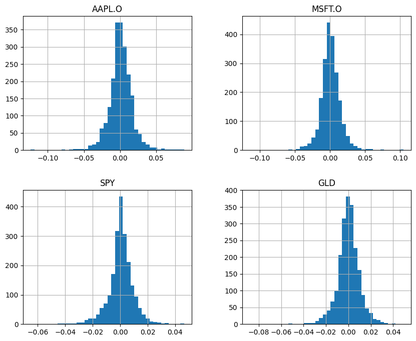
Let’s bring in our usual set of prices, pick four assets, calculate discrete returns, and plot a histogram of those returns.
We are going to use discrete (or simple, or arithmetic) returns instead of log returns, because we are doing portfolio optimization. In short, the return of a portfolio is the weighted average of the mean discrete returns. This is not true for mean log returns.
Important
Always use discrete (simple) returns when doing portfolio optimization. The portfolio return is the weighted sum of the individual asset discrete returns: \(R_p = \sum_i w_i R_i\). This additive property does not hold for log returns, which is why we don’t use them here.
# Read in some eod prices
import numpy as np
import pandas as pd

import matplotlib.pyplot as plt

# Include this to have plots show up in your Jupyter notebook.
%matplotlib inline

import scipy.optimize as sco

raw = pd.read_csv('https://raw.githubusercontent.com/aaiken1/fin-data-analysis-python/main/data/tr_eikon_eod_data.csv',
                  index_col=0, parse_dates=True).dropna()

symbols = ['AAPL.O', 'MSFT.O', 'SPY', 'GLD'] #two stocks and two ETFs

noa = len(symbols) #noa = number of assets

data = raw[symbols]

rets = data.pct_change().dropna()

rets.hist(bins=40, figsize=(10, 8));
rets.describe()
| AAPL.O | MSFT.O | SPY | GLD | |
|---|---|---|---|---|
| count | 2137.000000 | 2137.000000 | 2137.000000 | 2137.000000 |
| mean | 0.000969 | 0.000643 | 0.000452 | 0.000088 |
| std | 0.015900 | 0.014221 | 0.009313 | 0.010170 |
| min | -0.123549 | -0.113995 | -0.065123 | -0.087808 |
| 25% | -0.006883 | -0.006745 | -0.003418 | -0.005084 |
| 50% | 0.000667 | 0.000308 | 0.000580 | 0.000343 |
| 75% | 0.009597 | 0.007896 | 0.005071 | 0.005317 |
| max | 0.088741 | 0.104522 | 0.046499 | 0.049122 |
Note
These four return series each have the same number of observations. This is important when doing correlation and covariance matrices. You’ll likely want to just keep observations where none of the assets have missing returns. This is another reason why using historical data can be tricky - for a lot of specific assets, we just don’t have much data!
We can find the average daily return of each of these four sets of discrete returns and annualize them.
How should we do this? I am going to take the arithmetic mean (i.e. the usual average) and multiply by 252, the number of trading days in the year. This is a common way to go from daily to annual returns when doing portfolio optimization. This generalizes to monthly (12) and quarterly (4).
We’ll do the same thing when using the PyPortfolioOpt package. Note that this method does not take into account compounding. You could also annualize the arithmetic average of the monthly returns using geometric chaining, or \((1+mean)^{252}-1\). This will get you the annual return if you earned the mean daily return every day for 252 days. Finally, you could annualize the geometric mean of the daily returns using the same chaining principle. If you search around, you’ll find people doing all three.
rets.mean() * 252
AAPL.O    0.244313
MSFT.O    0.162139
SPY       0.113901
GLD       0.022214
dtype: float64
ann_rets = rets.mean() * 252
We’ll do something similar for our variance and covariance terms. We are going to take a short-cut and annualize the daily variances and covariances by multiplying by 252. You would annualize standard deviation by multiplying by \(\sqrt{252}\). Technically, you should only do this with log returns.
rets.cov() * 252
| AAPL.O | MSFT.O | SPY | GLD | |
|---|---|---|---|---|
| AAPL.O | 0.063710 | 0.023364 | 0.021015 | 0.001497 |
| MSFT.O | 0.023364 | 0.050965 | 0.022193 | -0.000337 |
| SPY | 0.021015 | 0.022193 | 0.021858 | 0.000041 |
| GLD | 0.001497 | -0.000337 | 0.000041 | 0.026063 |
Let’s save that somewhere. We’ll use it later.
ann_cov = rets.cov() * 252
ann_cov
| AAPL.O | MSFT.O | SPY | GLD | |
|---|---|---|---|---|
| AAPL.O | 0.063710 | 0.023364 | 0.021015 | 0.001497 |
| MSFT.O | 0.023364 | 0.050965 | 0.022193 | -0.000337 |
| SPY | 0.021015 | 0.022193 | 0.021858 | 0.000041 |
| GLD | 0.001497 | -0.000337 | 0.000041 | 0.026063 |
Note
You can also annualize everything at the end, after the optimization. The optimizer will work just fine with daily data, but you have to keep in mind that you’ll need a daily risk-free rate and that you’re finding a daily Sharpe ratio.
When you form a portfolio, you of course need to know how much of your portfolio is in each asset. Let’s pick some random weights to start. We’ll do that by choosing random numbers between 0 and 1. How many random numbers? The variable noa has the number of assets stored in it, so we’ll pick four. Then, we’ll divide each random number by the sum of the four numbers. This “trick” let’s us go from four numbers between 0 and 1 to four numbers that will add up to 1. Just like portfolio weights!
Note the /=. This divides every item in weights by the sum of the weights and then saves the result back to weights.
weights = np.random.random(noa)
weights /= np.sum(weights)
weights.sum()
1.0
Good! They add up to 1. Or, well, basically 1. Remember, computers try their best to store exact numbers, but there’s only so much precision that you can get.
np.sum(ann_rets * weights)
0.08238086272057653
We can also find portfolio variance using the random weights. Again, we’re annualizing variances and covariances.
np.dot(weights.T, np.dot(ann_cov, weights))
0.017981685680396813
Finally, we take the square root of variance to get standard deviation.
np.sqrt(np.dot(weights.T, np.dot(ann_cov, weights)))
0.1340958078405019
Ok, all of this was with random weights. Can we do any better than that, if we assume that our expected returns and variance-covariance matrix represent our best guess about how these assets will behave in the future? Note that this is a really big assumption. The past might not tell us much about the future.
Plotting the efficient frontier#
The efficient frontier represents the relationship between risk and return. Each point on the curve is the best return that you can get for a given level of risk. Or, equivalently, each point is the lowest risk that you can take for a particular expected return. We would expect to see a positive relationship between risk and return.
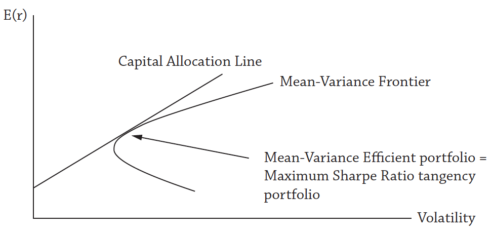
Fig. 56 The Capital Allocation Line, or CAL. The mean-variance frontier is the highest return you can get for a given level of risk. The CAL is all possible combinations have the highest Sharpe Ratio portfolio (the tangency portfolio) and the risk-free asset. If all investors have the same beliefs about all underlying assets, then they will all hold the same market portfolio, just in different quantities, depending on their risk preferences. Source: Asset Management by Andrew Ang#
What if we picked a bunch of random portfolios, found their risk and return, and then plotted each on a scatter plot? We should see the efficient frontier “emerge” as we essentially throw darts, since some risk-return combinations are not possible for a given set of assets. There’s only so much return you can get for a given level of risk.
To do this, let’s define two functions. One just takes weights and finds the portfolio return using the mean returns. The other finds the volatility of the portfolio using the weights passed to it. Note that both are just the formulas used above, but now in a function that we’ve defined.
How do you read the format of a user defined function? You use def to define the function name. Inside of (), you put the items that are getting passed, or given to, the function. In this case, whatever we give the function will be called weights inside of the function. What’s inside the function. You must end the first line with a :. Then, you need to indent everything that happens when the function is used. In this case, that’s just one line. The function will return whatever is on the line with return. In this case, the portfolio return and volatility.
def port_ret(weights):
    return np.sum(ann_rets * weights)
def port_vol(weights):
    return np.sqrt(np.dot(weights.T, np.dot(ann_cov, weights)))
Here’s the main part. We are going to use those two functions above to write some cleaner code. We start by creating two empty arrays, prets and pvols. We’ll then put a bunch of different portfolio mean returns and volatilities into these arrays. How are we going to get these different portfolio risk and return characteristics? Let’s create a bunch of random portfolios with random asset weights. In fact, let’s create 2500 random portfolios and see what each combination of risk and return looks like when we plot it. The shape should look familiar!
prets = []
pvols = []
for p in range (2500):
    weights = np.random.random(noa)
    weights /= np.sum(weights)
    prets.append(port_ret(weights))
    pvols.append(port_vol(weights))
prets = np.array(prets)
pvols = np.array(pvols)
The for statement will have the value p go from 0 to 2499 (i.e. 2500 times). For each of these times through the loop, we calculate our random weights and the portfolio returns and volatility for these weights, using the same expected returns and volatility for the assets each time through. Only the weights are changing. We then append, or stack, the return and volatility values on top of each other, creating two lists with 2500 numbers in them. But, we don’t want a list. We want an array of numbers. The last two lines convert the lists into numpy arrays which we can graph.
Let’s graph them. We’ll make a scatter plot with volatility on the x-axis and returns on the y-axis. The c= option adds a third dimension to the graph, where we pick a color for each dot based on another value. That value is the return for that dot divided by the volatility of that dot. In other words, darker red means bigger return over risk ratio, or larger Sharpe Ratio. Notice how the dark red is along the edge of the curve? This is the efficient frontier!
plt.figure(figsize=(10, 6))
plt.scatter(pvols, prets, c=prets / pvols,
            marker='o', cmap='coolwarm')
plt.xlabel('expected volatility')
plt.ylabel('expected return')
plt.colorbar(label='Sharpe ratio');
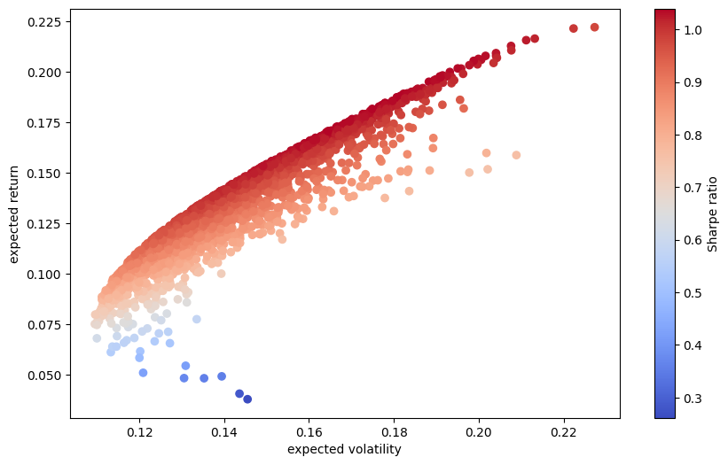
We’ve just generated the efficient frontier from a simulation. No “formulas”, per se. Just make 2500 random portfolios and at least some of them are going to be good!
Each portfolio on the envelope, the edge of the shape we see above, is on the efficient frontier. Each of these portfolios has the highest return for a given level of risk (or the lowest risk for a given return).
Important
The efficient frontier is the set of portfolios that offer the highest expected return for each level of risk. Any portfolio below the frontier is suboptimal – you could get more return for the same risk, or less risk for the same return, by moving to the frontier. Rational investors should only hold portfolios on the efficient frontier.
We’ll draw the efficient frontier below.
Optimizing#
Let’s use an optimizer to actually find the portfolio with the best Sharpe Ratio. This will be, for a given risk-free rate, the single portfolio with the best risk-reward trade-off.
We’ll also find the portfolio with the lowest volatility (risk). This portfolio is sometimes called the minimum variance portfolio.
We will assume in this example that the risk-free rate is zero. We are not subtracting the risk-free rate from the portfolio return in the numerator. Note that as you change the risk-free rate, you get different maximum Sharpe Ratio portfolios. What you’re doing, graphically, is tracing out the efficient frontier, finding different portfolios that are on the envelope.
Finding the max Sharpe portfolio#
We’ll start by defining a new function. This is our Sharpe Ratio. The optimization process that we’re going to use wants to find the minimum of something. So, we’ll make the Sharpe Ratio negative. This will then be the equivalent of finding the maximum.
def min_func_sharpe(weights):
    return -port_ret(weights) / port_vol(weights)
That’s the function that we are going to minimize. We are going to have Python find the weights that make that function as small as possible. Again, since the function has a negative sign in front, this is like finding the maximum.
Portfolio optimization always has a constraint where your weights must add up to one. To add this constraint, we are now going to set up a dictionary that our optimizer is going to be able to understand. The dictionary will say that we are going to give the optimizer something that is type eq, or an equation, and that the equation is the sum of all of our weights minus 1. The optimizer is going to know that we want this to be set equal to zero when solving for weights. In other words, all of our weights must add up to one - we are forcing the optimizer to do this.
Note
The optimizer interprets 'type': 'eq' as “this expression must equal zero.” So np.sum(x) - 1 = 0 means that all weights must sum to 1. You could also add inequality constraints with 'type': 'ineq', where the expression must be non-negative (greater than or equal to zero).
By the way, see the lambda x:? This is a lambda, or anonymous, function. These let us quickly and easily define a simple function. In this case, we have a function that is going to take an argument x and then do something with it. We are adding up all of the elements of x and then subtracting one. When we use this function, x will be our weights.
cons = ({'type': 'eq', 'fun': lambda x:  np.sum(x) - 1})
type(cons)
dict
We can now put some bounds on our weights. Weights, in this case, need to be between 0 and 1. This isn’t always the case! For example, short-selling means having weights less than 0. Leverage means weights greater than 1, potentially. To do this, we’ll create a tuple that has the set (0,1) for each asset in our portfolio, four in this case. This will tell the optimizer to keep each asset weight between 0 and 1.
bnds = tuple((0, 1) for x in range(noa))
bnds
((0, 1), (0, 1), (0, 1), (0, 1))
We’ll start by giving the optimizer an equally-weighted portfolio. It will change these weights to find the ones that minimize that negative Sharpe Ratio. This code will generate an array with equal weights, no matter how many assets you are using.
eweights = np.array(noa * [1. / noa])
eweights
array([0.25, 0.25, 0.25, 0.25])
By the way, here’s another way to do the same thing. I think I like this better.
eweights2 = np.full(noa, 1. / noa)
eweights2
array([0.25, 0.25, 0.25, 0.25])
Here’s the negative Sharpe Ratio with the equal-weights. So, the “real” Sharpe is 1.09.
min_func_sharpe(eweights)
-0.9936699253973043
Finally, let’s use the optimizer! We are going to use sco.minimize from the library SciPy, which we have brought in above. This function is like Solver in Excel. It is going to find the minimum value of some function by changing a set of variables in the function, subject to some constraints. The first argument is the function to minimize. The second argument is the initial guess. Then, we give it the method to use to find the minimum value. We’re using something called Sequential Least Squares Programming (SLSQP) here. Not important for us. We then give the optimizer our bounds for the variables and the constraints.
You can read more about this function in the SciPy manual here.
opts = sco.minimize(min_func_sharpe, eweights,
                    method='SLSQP', bounds=bnds,
                    constraints=cons)
type(opts)
scipy.optimize._optimize.OptimizeResult
We’ve saved the results in this OptimizeResult object. This object contains information about our optimization, including the optimal values it found. It calls these x - they are our weights that give us the minimum negative (i.e. maximum) Sharpe Ratio.
opts
     message: Optimization terminated successfully
     success: True
      status: 0
         fun: -1.039672055954719
           x: [ 5.011e-01  2.379e-01  1.445e-01  1.165e-01]
         nit: 7
         jac: [-6.109e-06 -2.135e-04  5.583e-05  3.933e-04]
        nfev: 35
        njev: 7
 multipliers: [ 5.632e-05]
Let’s pull out just the weights from the object and round to three decimal places.
opts['x'].round(3)
array([0.501, 0.238, 0.144, 0.116])
Here’s the portfolio return with those weights.
port_ret(opts['x']).round(3)
0.18
And the portfolio volatility with those weights.
port_vol(opts['x']).round(3)
0.173
And, the Sharpe Ratio with those weights.
port_ret(opts['x']) / port_vol(opts['x'])
1.039672055954719
Finding the minimum variance portfolio.#
We can do the same things and find the set of weights that minimize portfolio variance. Instead of minimizing the negative of the Sharpe Ratio, we’ll minimize the function that contains the formula for portfolio volatility, port_vol.
optv = sco.minimize(port_vol, eweights,
                    method='SLSQP', bounds=bnds,
                    constraints=cons)
optv
     message: Optimization terminated successfully
     success: True
      status: 0
         fun: 0.10912534155373545
           x: [ 0.000e+00  0.000e+00  5.438e-01  4.562e-01]
         nit: 9
         jac: [ 1.110e-01  1.092e-01  1.091e-01  1.092e-01]
        nfev: 45
        njev: 9
 multipliers: [ 1.091e-01]
optv['x'].round(3)
array([0. , 0. , 0.544, 0.456])
Nothing in our first asset, Apple. Since we are just minimizing variance, we don’t care about Apple’s nice return over this period.
We can find the Sharpe Ratio for the minimum variance portfolio. Note how it is lower!
Also, finding minimum variance and minimum volatility are the same thing, since volatility is just the square root of variance.
Note
The minimum variance portfolio is interesting because it only depends on the covariance matrix – it doesn’t use expected returns at all. Since expected returns are notoriously hard to estimate, some practitioners prefer the minimum variance portfolio precisely because it avoids this estimation problem. Research has shown that minimum variance portfolios often perform surprisingly well out-of-sample.
port_vol(optv['x']).round(3)
0.109
port_ret(optv['x']).round(3)
0.072
port_ret(optv['x']) / port_vol(optv['x'])
0.660505302399435
Efficient Frontier#
Let’s now trace out the actual efficient frontier. We are going to follow an “algorithm”, so to speak. Here are the steps:
Pick a target return.
Find the portfolio that gives you the minimum portfolio standard deviation (volatility) for that target return.
Repeat this process for a large number of target returns.
These steps will find a bunch of different portfolios, all that live on the envelope of the set containing all of the possible portfolios. These are the portfolios on the efficient frontier.
To do this, we now need two constraints. First, we want our portfolio return to be equal to some target return, tret. Second, we again have our weights must sum to one constraint.
Both of these constraints can live inside of the cons tuple. This tuple contains two dictionaries. Kind of confusing, but we just need to understand the syntax for writing out different constraints. The only part that changes is the code after lambda x:.
cons = ({'type': 'eq', 'fun': lambda x:  port_ret(x) - tret},
        {'type': 'eq', 'fun': lambda x:  np.sum(x) - 1})
type(cons)
tuple
Our bounds again, same as before.
bnds = tuple((0, 1) for x in range(noa))
Let’s create an array of values from 0.05 to 0.20. This represents a minimum of a 5% return and a maximum of a 20% return. We’ll do 50 evenly-spaced values. Each one of these represents one target return. We are going to find and store the minimum volatility that gives us each return.
trets = np.linspace(0.05, 0.2, 50)
print(type(trets))
trets
<class 'numpy.ndarray'>
array([0.05      , 0.05306122, 0.05612245, 0.05918367, 0.0622449 ,
       0.06530612, 0.06836735, 0.07142857, 0.0744898 , 0.07755102,
       0.08061224, 0.08367347, 0.08673469, 0.08979592, 0.09285714,
       0.09591837, 0.09897959, 0.10204082, 0.10510204, 0.10816327,
       0.11122449, 0.11428571, 0.11734694, 0.12040816, 0.12346939,
       0.12653061, 0.12959184, 0.13265306, 0.13571429, 0.13877551,
       0.14183673, 0.14489796, 0.14795918, 0.15102041, 0.15408163,
       0.15714286, 0.16020408, 0.16326531, 0.16632653, 0.16938776,
       0.17244898, 0.1755102 , 0.17857143, 0.18163265, 0.18469388,
       0.1877551 , 0.19081633, 0.19387755, 0.19693878, 0.2       ])
And here’s the optimization process. We start with an empty array that will eventually contain 50 different volatilities (standard deviations). Then, we loop through each target return in trets. Each one gets stored in tret and used in the For loop. The optimizer uses that target return as part of the constraint function that we included. We are then storing the value of the minimized portfolio volatility function in tvols. Note that we are not storing the weights for each portfolio. We only care about the minimum volatilities for each return.
%%time
tvols = []
for tret in trets:
    res = sco.minimize(port_vol, eweights, method='SLSQP',
                       bounds=bnds, constraints=cons)
    tvols.append(res['fun'])
tvols = np.array(tvols)
CPU times: user 401 ms, sys: 35.9 ms, total: 437 ms
Wall time: 214 ms
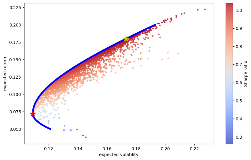
And now we can plot our efficient frontier. The efficient frontier is each target return, minimum volatility pair. That blue line is the frontier and is being added by the first plt.plot statement. The second plt.plot adds the yellow star at the max Sharpe Ratio portfolio. The third plt.plot adds the red star at the global minimum variance portfolio. Notice how both of these are pulling the weights, x, out of their respective Optimizer objects.
plt.figure(figsize=(10, 6))
plt.scatter(pvols, prets, c=prets / pvols,
            marker='.', alpha=0.8, cmap='coolwarm')
plt.plot(tvols, trets, 'b', lw=4.0)
plt.plot(port_vol(opts['x']), port_ret(opts['x']),
         'y*', markersize=15.0)
plt.plot(port_vol(optv['x']), port_ret(optv['x']),
         'r*', markersize=15.0)
plt.xlabel('expected volatility')
plt.ylabel('expected return')
plt.colorbar(label='Sharpe ratio');
PyPortfolioOpt#
To get started, you’ll need to type pip install PyPortfolioOpt in your Terminal below. This will install the package, since it doesn’t come with Anaconda. We can then bring in what we need.
You can read all about the PyPortfolioOpt package here.
You can also find examples on the author’s Github page. The creator of this package is a recent Cambridge graduate, not much older than you.
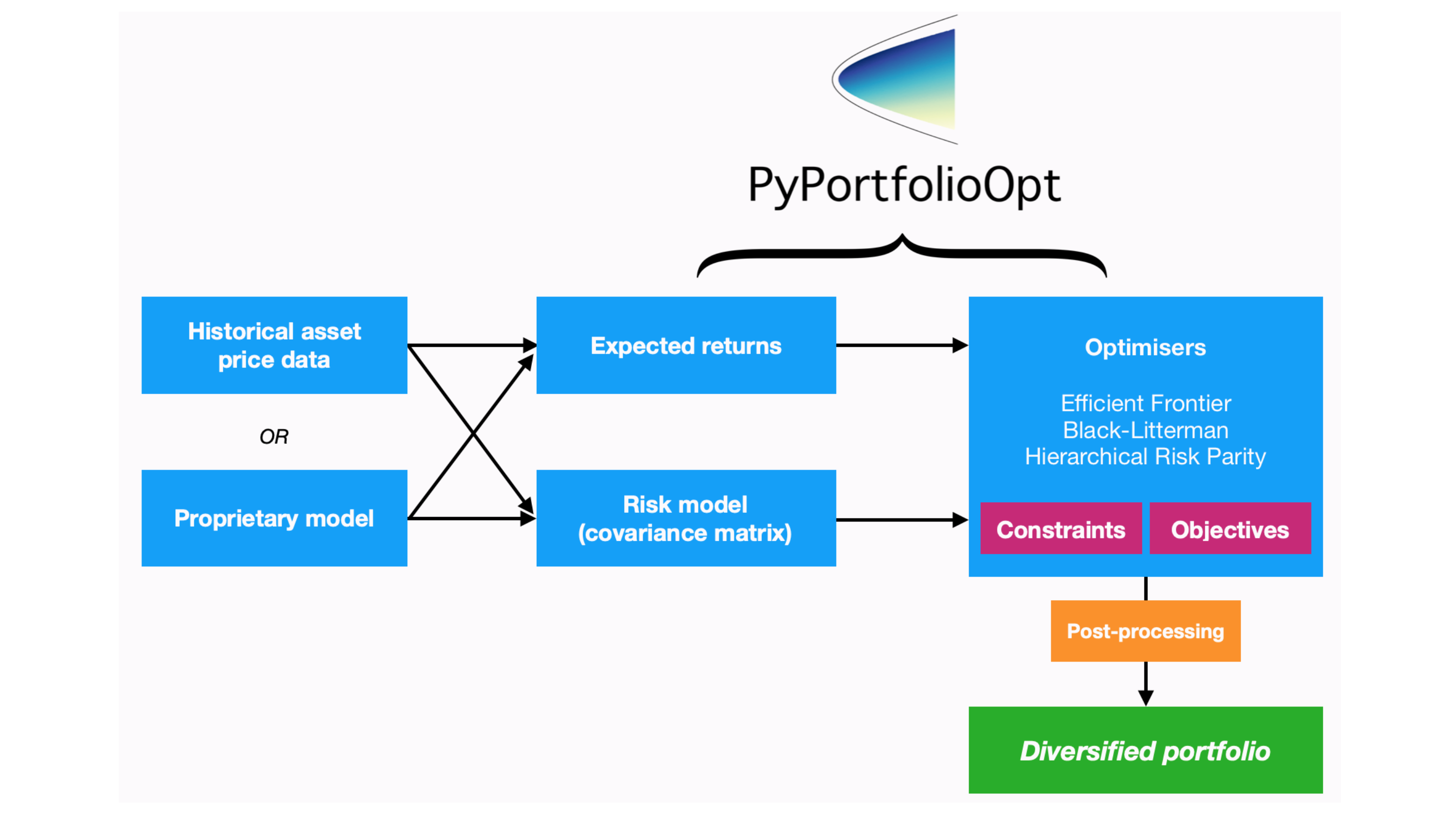
Fig. 57 The portfolio optimization process. Source: PyPortfolioOpt#
This page takes the explanations on the Github page and provides some nicer formatting.
from pypfopt.efficient_frontier import EfficientFrontier
from pypfopt import risk_models, expected_returns, plotting
We can find expected returns and the sample variance-covariance matrix using functions from PyPortfolioOpt. Notice that these functions want prices, not returns, by default. So, I’m using the DataFrame data, not ret. You can change this setting with the argument returns_data = True.
I’ll start by finding returns from prices.
rets_pyp = expected_returns.returns_from_prices(data)
rets_pyp
| AAPL.O | MSFT.O | SPY | GLD | |
|---|---|---|---|---|
| Date | ||||
| 2010-01-05 | 0.001729 | 0.000323 | 0.002647 | -0.000911 |
| 2010-01-06 | -0.015906 | -0.006137 | 0.000704 | 0.016500 |
| 2010-01-07 | -0.001849 | -0.010335 | 0.004221 | -0.006188 |
| 2010-01-08 | 0.006648 | 0.006830 | 0.003328 | 0.004963 |
| 2010-01-11 | -0.008822 | -0.012720 | 0.001397 | 0.013289 |
| ... | ... | ... | ... | ... |
| 2018-06-25 | -0.014871 | -0.020118 | -0.013613 | -0.003739 |
| 2018-06-26 | 0.012406 | 0.007013 | 0.002214 | -0.005255 |
| 2018-06-27 | -0.001464 | -0.015543 | -0.008284 | -0.005702 |
| 2018-06-28 | 0.007276 | 0.011175 | 0.005717 | -0.003036 |
| 2018-06-29 | -0.002102 | -0.000203 | 0.001440 | 0.003637 |
2137 rows × 4 columns
rets
| AAPL.O | MSFT.O | SPY | GLD | |
|---|---|---|---|---|
| Date | ||||
| 2010-01-05 | 0.001729 | 0.000323 | 0.002647 | -0.000911 |
| 2010-01-06 | -0.015906 | -0.006137 | 0.000704 | 0.016500 |
| 2010-01-07 | -0.001849 | -0.010335 | 0.004221 | -0.006188 |
| 2010-01-08 | 0.006648 | 0.006830 | 0.003328 | 0.004963 |
| 2010-01-11 | -0.008822 | -0.012720 | 0.001397 | 0.013289 |
| ... | ... | ... | ... | ... |
| 2018-06-25 | -0.014871 | -0.020118 | -0.013613 | -0.003739 |
| 2018-06-26 | 0.012406 | 0.007013 | 0.002214 | -0.005255 |
| 2018-06-27 | -0.001464 | -0.015543 | -0.008284 | -0.005702 |
| 2018-06-28 | 0.007276 | 0.011175 | 0.005717 | -0.003036 |
| 2018-06-29 | -0.002102 | -0.000203 | 0.001440 | 0.003637 |
2137 rows × 4 columns
We can compare that with our original return file and see that this function is calculating discrete returns by default, since the returns are the same. We can use the package to find annualized returns too. I’ll give the function the price data again. I will also set compounding to False, as we don’t typically use annualized geometric means (CAGRs) for portfolio optimization. I want arithmetic means. The default for this function is that you have daily returns, or 252 time periods.
However, the annualization simply takes the monthly arithmetic mean and multiplies by 252. This is why the average returns we’re using are lower than the ones above.
But, I’ll add each option, just so that you can that they are there.
mu = expected_returns.mean_historical_return(data, compounding = False, log_returns = False, frequency = 252)
mu
AAPL.O    0.244313
MSFT.O    0.162139
SPY       0.113901
GLD       0.022214
dtype: float64
You can actually see the code for these functions. I like looking through code like this to both learn what these functions are doing, what my options are, etc., as well as learning how to write better Python myself!
You can see how the function is getting the annual returns by just multiplying by 252, the number of trading days.
rets.mean()*252
AAPL.O    0.244313
MSFT.O    0.162139
SPY       0.113901
GLD       0.022214
dtype: float64
The package author has a good comment in his documents about the issues with using historical data for returns:
This is probably the default textbook approach. It is intuitive and easily interpretable, however the estimates are subject to large uncertainty. This is a problem especially in the context of a mean-variance optimizer, which will maximise the erroneous inputs.
In other words, the assets with the largest historical returns are likely the assets with the greatest estimation error. But, the simplest optimization methods, like what we’re doing, will choose those assets! And, the same is true for the worst performing assets. Their negative performance might be exaggerated too.
Warning
Mean-variance optimization is notoriously sensitive to its inputs, especially expected returns. Small changes in expected returns can lead to wildly different optimal portfolios. This is sometimes called the “error maximization” problem. In practice, practitioners use techniques like shrinkage (e.g., Ledoit-Wolf), Black-Litterman models, or constraints on position sizes to produce more stable, reasonable portfolios. The PyPortfolioOpt package supports many of these approaches.
Next, we can create and store the sample variance-covariance matrix. “Sample” means that we are using sample variance and covariance (as opposed to population variance and covariance).
S = risk_models.sample_cov(data)
S
| AAPL.O | MSFT.O | SPY | GLD | |
|---|---|---|---|---|
| AAPL.O | 0.063710 | 0.023364 | 0.021015 | 0.001497 |
| MSFT.O | 0.023364 | 0.050965 | 0.022193 | -0.000337 |
| SPY | 0.021015 | 0.022193 | 0.021858 | 0.000041 |
| GLD | 0.001497 | -0.000337 | 0.000041 | 0.026063 |
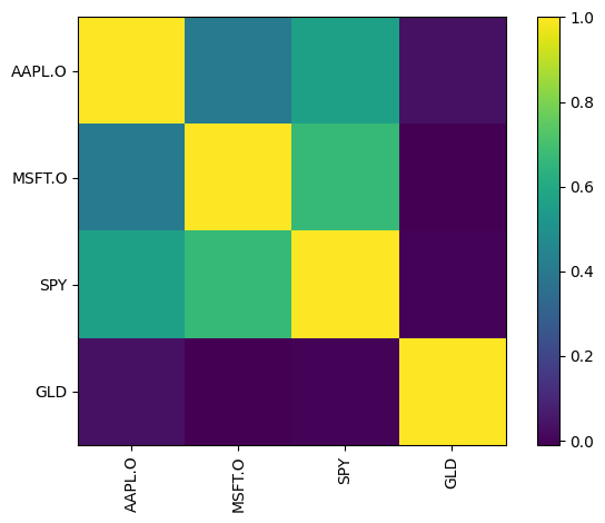
PyPortfolioOpt has built-in plotting functions that create matplotlib plots, among other plot types. Here’s one showing the correlations among our four assets. Gold immediately stands out.
plotting.plot_covariance(S, plot_correlation=True)
<Axes: >
Let’s find our max Sharpe portfolio. We’ll do this step-by-step. First, we’ll use the function EfficientFrontier to find and create an object that contains the information needed to describe the efficient frontier for these assets. Note that you just need the expected returns and the variance-covariance matrix to define the efficient frontier.
ef = EfficientFrontier(mu, S)
ef
<pypfopt.efficient_frontier.efficient_frontier.EfficientFrontier at 0x132430a40>
This ef object contains useful things. For example, it let’s us pull our the max Sharpe portfolio for a given risk-free rate. Remember, you pick a risk-free rate and draw that tangency line over to the efficient frontier. So, different assumed risk-free rates give you different max Sharpe portfolios.
raw_weights = ef.max_sharpe(risk_free_rate = 0.025)
raw_weights
OrderedDict([('AAPL.O', 0.6881492096432079),
             ('MSFT.O', 0.3118507903567919),
             ('SPY', 0.0),
             ('GLD', 0.0)])
This comes out as a type of Dictionary. We can use clean_weights() to get rid of some of the decimal places.
cleaned_weights = ef.clean_weights()
cleaned_weights
OrderedDict([('AAPL.O', 0.68815),
             ('MSFT.O', 0.31185),
             ('SPY', 0.0),
             ('GLD', 0.0)])
Finally, we can pull out the return and risk characteristics of this max Sharpe portfolio with that assumed risk-free rate.
perf = ef.portfolio_performance(verbose=True, risk_free_rate = 0.025)
perf
Expected annual return: 21.9%
Annual volatility: 21.2%
Sharpe Ratio: 0.91
(0.21868665539725823, 0.21249455919923924, 0.9114899512116622)
You can even access the individual values in this perf tuple I created. Here’s the expected annual return
type(perf)
tuple
perf[0]
0.21868665539725823
This package does much more than this. I encourage you to take a look! Here’s one additional example, with two changes. First, I’ve added some weight bounds for the assets added to the EfficientFrontier method. Second, instead of finding the max Sharpe portfolio, I’m using ef.efficient_return to find the portfolio with the least amount of risk that gives a target return of 18%.
You can see from the output below that we did indeed hit our target return.
See how Apple hits the upper limit I set of 50%? Apple did so well during this period that the optimizer really wants us to put most of our money in it. Is that a good idea?
Important
This is why weight constraints are so important in practice. Without them, the optimizer will concentrate your portfolio in whatever asset had the best historical performance. But past performance is not a reliable predictor of future returns. Constraints force diversification and produce more robust portfolios. The weight_bounds parameter also allows negative weights (short selling) if you set the lower bound below zero, as I’ve done here with -0.2.
ef = EfficientFrontier(mu, S, weight_bounds=(-0.2, 0.5))
raw_weights = ef.efficient_return(target_return = 0.18, market_neutral=False)
cleaned_weights = ef.clean_weights()
print(cleaned_weights)
ef.portfolio_performance(verbose=True)
OrderedDict({'AAPL.O': 0.5, 'MSFT.O': 0.2387, 'SPY': 0.14546, 'GLD': 0.11584})
Expected annual return: 18.0%
Annual volatility: 17.3%
Sharpe Ratio: 1.04
(0.17999999999999997, 0.1731317071656996, 1.0396709126637729)