
FRED API#
The Federal Reserve Economic Data (FRED) is maintained by the Federal Reserve Bank of St. Louis. It contains over 800,000 economic time series from dozens of sources, including:
GDP and economic growth indicators
Inflation measures (CPI, PCE)
Interest rates and yield curves
Employment and labor market data
International economic data
Cryptocurrency prices
Getting Started with FRED#
To use the FRED API, you need to:
Create a FRED account
Request an API key
Store your key securely (never hardcode it!)
Install the package:
pip install fredapi
Set-up#
# Core packages
from fredapi import Fred
import os
from dotenv import load_dotenv

import numpy as np
import pandas as pd
import datetime as dt

import matplotlib as mpl
import matplotlib.pyplot as plt

# Include this to have plots show up in your Jupyter notebook.
%matplotlib inline
# Load API keys from .env file
load_dotenv()

# Retrieve API keys
FRED_API_KEY = os.getenv('FRED_API_KEY')

# Initialize FRED API
fred = Fred(api_key=FRED_API_KEY)
Secure API Key Storage#
Here’s the wrong way to use your API key:
# DON'T DO THIS!
fred = Fred(api_key='your_api_key_here')
If you push this code to GitHub, your key is exposed to the world!
Using a .env File (Recommended for Local Development)#
A .env file is a simple text file that stores your API keys as key-value pairs. It lives in your project folder but is never committed to GitHub.
Step 1: Create a file called .env in your project’s root folder (the same folder as your notebooks). You can do this in VS Code or any text editor. The file contents look like this:
FRED_API_KEY=your_actual_key_here
No quotes, no spaces around the =. Just the variable name and the key.
Step 2: Make sure .env is in your .gitignore file so it doesn’t get pushed to GitHub:
# .gitignore
.env
Step 3: In your Python code, use python-dotenv to load the key:
from dotenv import load_dotenv
import os

load_dotenv()  # Reads the .env file and loads variables into the environment
FRED_API_KEY = os.getenv('FRED_API_KEY')

fred = Fred(api_key=FRED_API_KEY)
load_dotenv() reads the .env file and makes its variables available through os.getenv(). This is exactly what our set-up cell above does.
Note
Install python-dotenv if you don’t have it: pip install python-dotenv
Using GitHub Secrets (Recommended for Codespaces)#
If you’re using GitHub Codespaces, you can store keys as Codespace Secrets instead of a .env file. These are encrypted and automatically available as environment variables inside your Codespace.
Here’s how to add a secret:
Go to github.com and click your profile picture in the upper-right corner
Click Settings
In the left sidebar, scroll down to the “Code, planning, and automation” section and click Codespaces
Next to “Codespaces secrets”, click New secret
In the Name field, type your secret name (e.g.,
FRED_API_KEY)In the Value field, paste your API key
Click the Repository access dropdown and select the repo(s) that should have access to this secret
Click Add secret
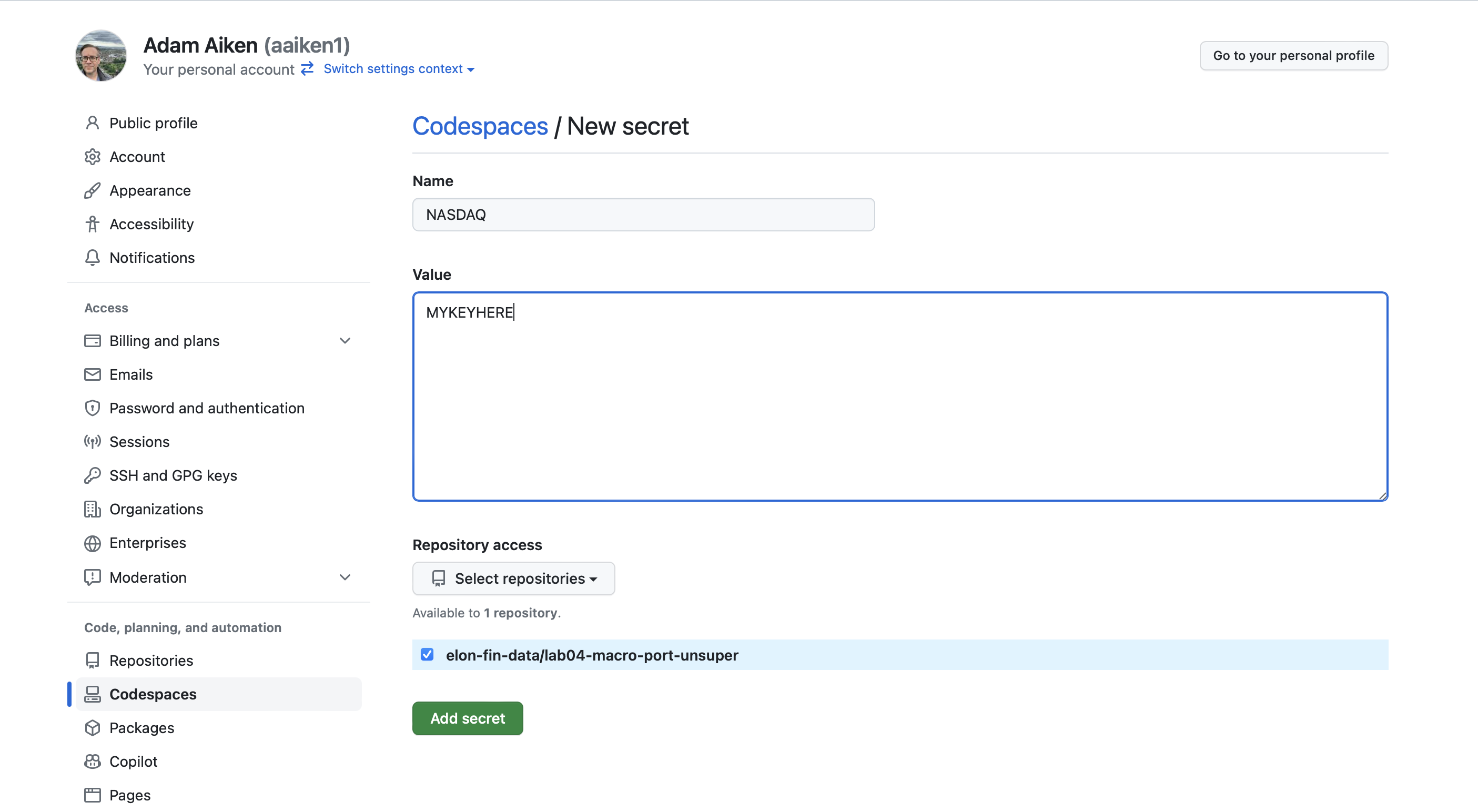
Fig. 40 GitHub Codespaces secrets settings.#
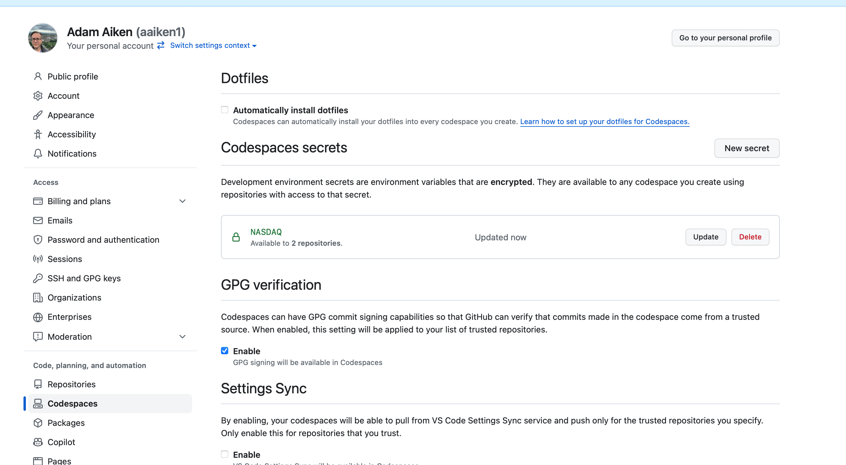
Fig. 41 Adding a new secret.#
Codespace Secrets are automatically available as environment variables, so you can access them the same way:
FRED_API_KEY = os.getenv('FRED_API_KEY')
fred = Fred(api_key=FRED_API_KEY)
You don’t need load_dotenv() for Codespace Secrets, but it doesn’t hurt to include it – if no .env file exists, it just does nothing.
Troubleshooting GitHub Secrets#
If your code can’t find your API key (e.g., you get an error like ValueError or None when you try to use it), work through this checklist:
1. Check your secret name for typos. The name you use in os.getenv('FRED_API_KEY') must exactly match the name you entered on GitHub. Secret names are not case-sensitive on GitHub’s side, but it’s good practice to keep them consistent. Only letters, numbers, and underscores are allowed – no spaces or special characters.
2. Check the API key value itself. When you paste your key into the Value field on GitHub, make sure you haven’t accidentally copied extra spaces or characters before or after the key. A trailing space or newline character will silently break things.
3. Make sure you granted repository access. When you created the secret, you needed to select which repositories can use it. If you forgot to add your lab repo, the secret won’t be available in that Codespace. Go back to Settings > Codespaces > Codespaces secrets, click on the secret name, and make sure your repo is listed under repository access.
4. Stop and restart your Codespace. Secrets are loaded when a Codespace starts up. If you added or changed a secret while your Codespace was already running, it won’t pick up the change automatically. You need to stop the Codespace and then reopen it. Here’s how:
Save your work first. Do a
git add,git commit, andgit push(or use the Source Control panel in VS Code to sync) so your files are backed up to GitHub.Close the Codespace browser tab (or VS Code window). Note that closing the tab alone does not stop the Codespace – it keeps running in the background.
Go to github.com/codespaces. This page lists all of your Codespaces.
Find the Codespace you want to restart. Click the three dots (
...) to the right of it.Click Stop codespace.
Once it has stopped, go back to your lab repository on GitHub and click the green Code button, then Codespaces, and open your existing Codespace. It will restart with the updated secrets.
5. Verify the secret is loaded. You can add a quick check in your notebook to make sure the key was found (without printing the actual key!):
FRED_API_KEY = os.getenv('FRED_API_KEY')
print(type(FRED_API_KEY))  # Should print <class 'str'>, not <class 'NoneType'>
If it prints <class 'NoneType'>, the secret isn’t being found. Go back through the steps above.
FRED Example: Bitcoin Data#
Let’s pull Bitcoin price data from FRED. You can find the series here.
When you find data on FRED, note the series code - that’s how you’ll request it via the API.
btc = fred.get_series('CBBTCUSD')
btc.tail()
2026-03-06    68350.00
2026-03-07    67193.87
2026-03-08    66055.14
2026-03-09    68480.54
2026-03-10    69847.95
dtype: float64
That’s just a plain Series, not a DataFrame. Let’s convert it and clean it up.
btc = btc.to_frame(name='btc')
btc = btc.rename_axis('date')
btc
| btc | |
|---|---|
| date | |
| 2014-12-01 | 370.00 |
| 2014-12-02 | 378.00 |
| 2014-12-03 | 378.00 |
| 2014-12-04 | 377.10 |
| 2014-12-05 | NaN |
| ... | ... |
| 2026-03-06 | 68350.00 |
| 2026-03-07 | 67193.87 |
| 2026-03-08 | 66055.14 |
| 2026-03-09 | 68480.54 |
| 2026-03-10 | 69847.95 |
4118 rows × 1 columns
# Drop missing values
btc = btc.dropna()
# Calculate returns
btc['ret'] = btc['btc'].pct_change()
/var/folders/kx/y8vj3n6n5kq_d74vj24jsnh40000gn/T/ipykernel_31063/1503532820.py:2: SettingWithCopyWarning:
A value is trying to be set on a copy of a slice from a DataFrame.
Try using .loc[row_indexer,col_indexer] = value instead

See the caveats in the documentation: https://pandas.pydata.org/pandas-docs/stable/user_guide/indexing.html#returning-a-view-versus-a-copy
  btc['ret'] = btc['btc'].pct_change()
btc = btc.loc['2015-01-01':, ['btc', 'ret']]
btc.plot()
<Axes: xlabel='date'>
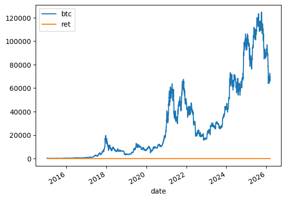
That’s not a very good graph - the returns and price levels are in different units. Let’s format the average return nicely:
print(f'Average return: {100 * btc.ret.mean():.2f}%')
Average return: 0.20%
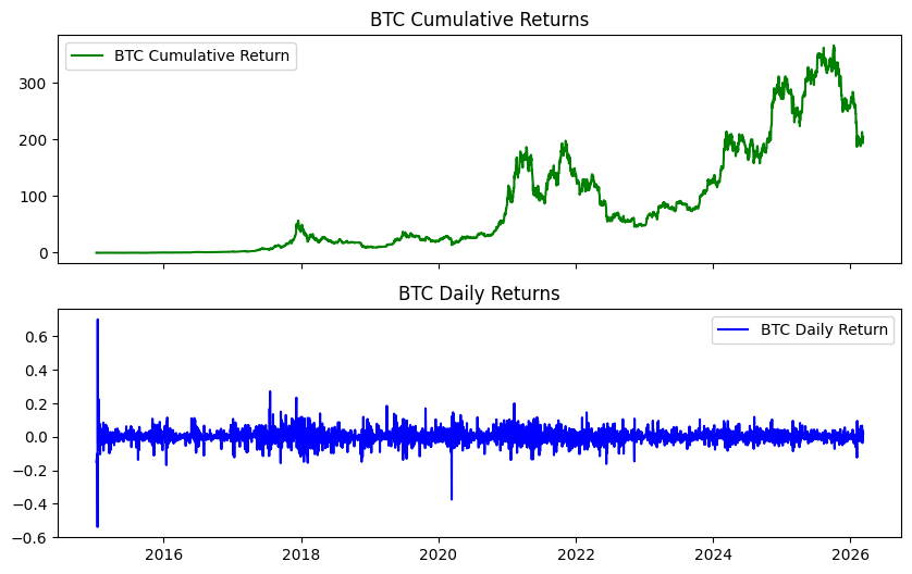
Visualizing Cumulative Returns#
Let’s create a cumulative return chart and daily return chart, stacked on top of each other.
btc['ret_g'] = btc.ret.add(1)  # gross return
btc['ret_c'] = btc.ret_g.cumprod().sub(1)  # cumulative return
btc
| btc | ret | ret_g | ret_c | |
|---|---|---|---|---|
| date | ||||
| 2015-01-08 | 288.99 | -0.150029 | 0.849971 | -0.150029 |
| 2015-01-13 | 260.00 | -0.100315 | 0.899685 | -0.235294 |
| 2015-01-14 | 120.00 | -0.538462 | 0.461538 | -0.647059 |
| 2015-01-15 | 204.22 | 0.701833 | 1.701833 | -0.399353 |
| 2015-01-16 | 199.46 | -0.023308 | 0.976692 | -0.413353 |
| ... | ... | ... | ... | ... |
| 2026-03-06 | 68350.00 | -0.036720 | 0.963280 | 200.029412 |
| 2026-03-07 | 67193.87 | -0.016915 | 0.983085 | 196.629029 |
| 2026-03-08 | 66055.14 | -0.016947 | 0.983053 | 193.279824 |
| 2026-03-09 | 68480.54 | 0.036718 | 1.036718 | 200.413353 |
| 2026-03-10 | 69847.95 | 0.019968 | 1.019968 | 204.435147 |
4074 rows × 4 columns
fig, axs = plt.subplots(2, 1, sharex=True, sharey=False, figsize=(10, 6))

axs[0].plot(btc.ret_c, 'g', label='BTC Cumulative Return')
axs[1].plot(btc.ret, 'b', label='BTC Daily Return')

axs[0].set_title('BTC Cumulative Returns')
axs[1].set_title('BTC Daily Returns')

axs[0].legend()
axs[1].legend();
A Bitcoin Simulation #
Let’s put together some ideas, write a function, and run a simulation using Geometric Brownian Motion (GBM).
What is GBM?#
GBM is a stochastic differential equation commonly used to model asset prices:
This says the change in stock price has two components:
A drift (\(\mu\)): the average increase over time
A shock (\(\sigma dW_t\)): random noise scaled by volatility
The solution gives us the price at any time \(t\):
Note
We’re not predicting here. We’re capturing basic dynamics of how an asset moves and seeing what’s possible in the future.
# Simulation parameters
T = 30        # Time horizon (days)
N = 30        # Number of time steps
S_0 = btc.btc.iloc[-1]  # Initial BTC price
N_SIM = 100   # Number of simulations
mu = btc.ret.mean()
sigma = btc.ret.std()
def simulate_gbm(s_0, mu, sigma, n_sims, T, N):
    """Simulate asset prices using Geometric Brownian Motion."""
    dt = T / N  # One day
    dW = np.random.normal(scale=np.sqrt(dt), size=(n_sims, N))  # Random shocks
    W = np.cumsum(dW, axis=1)  # Cumulative sum of shocks
    time_step = np.linspace(dt, T, N)
    time_steps = np.broadcast_to(time_step, (n_sims, N))
    S_t = s_0 * np.exp((mu - 0.5 * sigma ** 2) * time_steps + sigma * np.sqrt(time_steps) * W)
    S_t = np.insert(S_t, 0, s_0, axis=1)
    return S_t
# Run the simulation
gbm_simulations = simulate_gbm(S_0, mu, sigma, N_SIM, T, N)
# Plot all simulations
gbm_simulations_df = pd.DataFrame(np.transpose(gbm_simulations))

ax = gbm_simulations_df.plot(alpha=0.2, legend=False)
ax.set_title('BTC Price Simulations (30 days)', fontsize=16)
ax.set_xlabel('Days')
ax.set_ylabel('Price ($)');
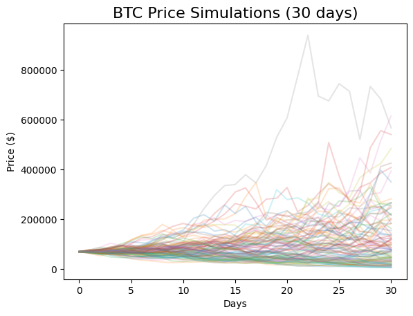
The y-axis has a wide range because some extreme values are possible given Bitcoin’s high volatility.
FRED Example: GDP Data#
Let’s pull another common series - U.S. GDP. The series code is GDP.
gdp = fred.get_series('GDP', observation_start='2010-01-01', observation_end='2023-01-27')
gdp = gdp.to_frame(name='GDP')
gdp.head()
| GDP | |
|---|---|
| 2010-01-01 | 14764.610 |
| 2010-04-01 | 14980.193 |
| 2010-07-01 | 15141.607 |
| 2010-10-01 | 15309.474 |
| 2011-01-01 | 15351.448 |
You can browse available series on the FRED website and use their series codes with fred.get_series(). Check the fredapi documentation for more options, like searching for series by keyword.