From Regression to Prediction: Can ML Beat the Market?

We have now covered OLS regression, Lasso, Ridge, and Elastic Net. We have learned about train/test splits, cross-validation, and hyperparameter tuning. The natural next question: can we use these tools to predict stock returns?

The short answer is humbling. Let’s walk through what actually happens when you take these models to financial markets.

The model horse race

A common exercise in machine learning is the model horse race – train several models on the same data and compare their performance. When researchers do this with stock market data (e.g., predicting whether the S&P 500 goes up or down), a striking pattern emerges.

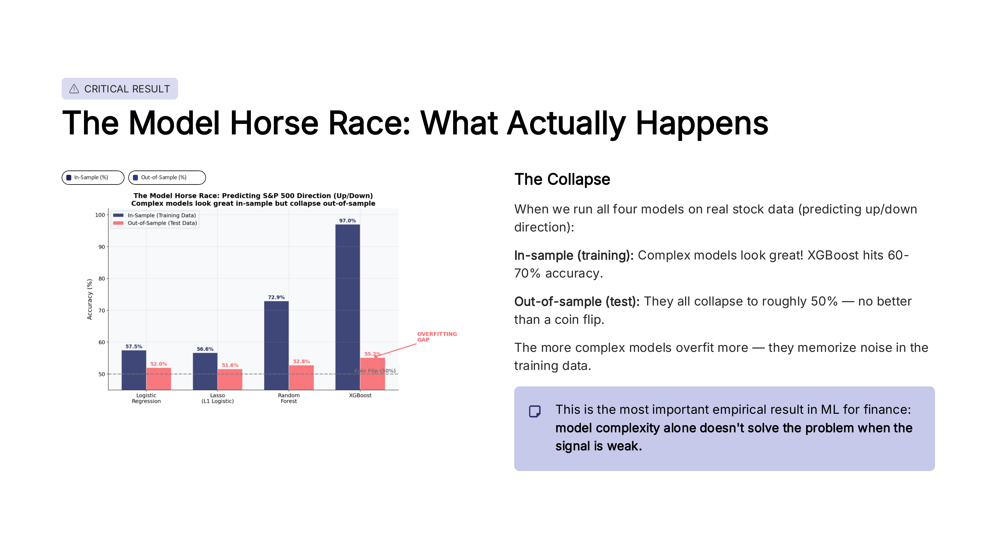
Fig. 93 The model horse race: predicting S&P 500 direction. Complex models look great in-sample but collapse out-of-sample. Source: Professor Jonathan Hersh, BUS 696: Generative AI in Finance, Chapman University, Spring 2026.

Look at the pattern in the figure. In-sample (training data), more complex models do better – Lasso beats logistic regression, and tree-based models beat Lasso. XGBoost can hit 97% accuracy in the training data! But out-of-sample (test data), they all collapse to roughly 50% – no better than a coin flip.

The more complex the model, the larger the gap between training and test accuracy. This gap is the overfitting. XGBoost memorized the training data perfectly, but learned nothing that generalizes to new data.

Important

This is the most important empirical result in financial ML: model complexity alone does not solve the problem when the signal is weak. Financial returns have an extremely low signal-to-noise ratio. No amount of model sophistication can extract a signal that isn’t there.

What ~52% accuracy actually looks like

Even the best academic models for predicting market direction tend to land around 51-53% accuracy. That sounds close to 50%, but is it meaningfully different? Let’s look at what this means in practice.

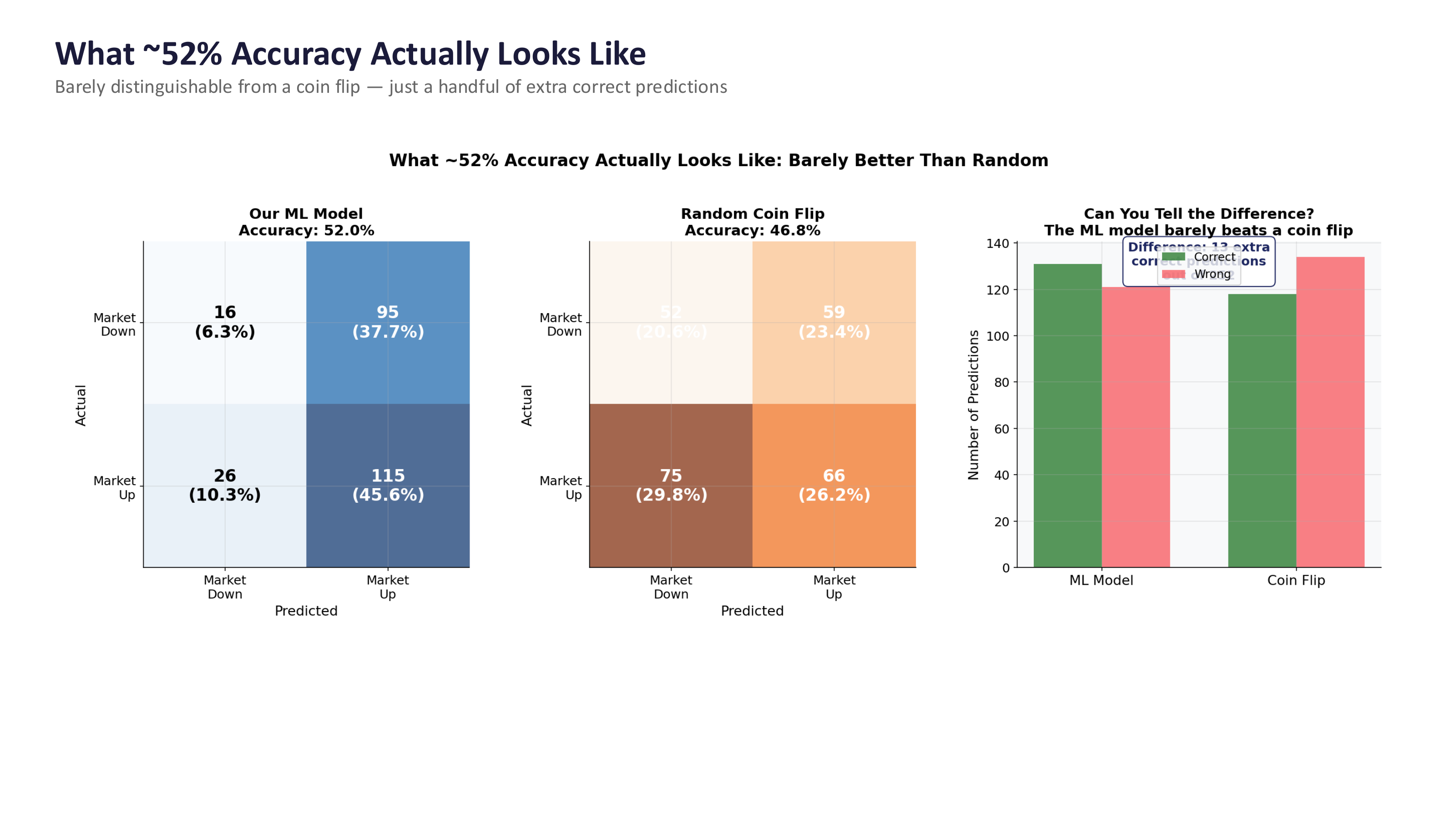
Fig. 94 What ~52% accuracy actually looks like compared to a coin flip. The confusion matrices are nearly identical. Source: Professor Jonathan Hersh, BUS 696: Generative AI in Finance, Chapman University, Spring 2026.

The figure compares an ML model at 52% accuracy to a random coin flip at ~47%. The confusion matrices look almost identical. The bar chart on the right makes it even clearer – the ML model gets just a handful of extra correct predictions compared to pure randomness.

This is a sobering result. After all of the modeling effort – feature engineering, cross-validation, hyperparameter tuning – you end up barely distinguishable from a coin flip. But here is the key insight: in finance, even a tiny edge can be enormously valuable if you know how to exploit it. The question is not just can you predict? but what do you do with that prediction?

What the smart money actually does

If model complexity alone doesn’t work, how does anyone make money with ML in finance? The answer is that successful quantitative firms approach the problem very differently from a standard Kaggle competition.

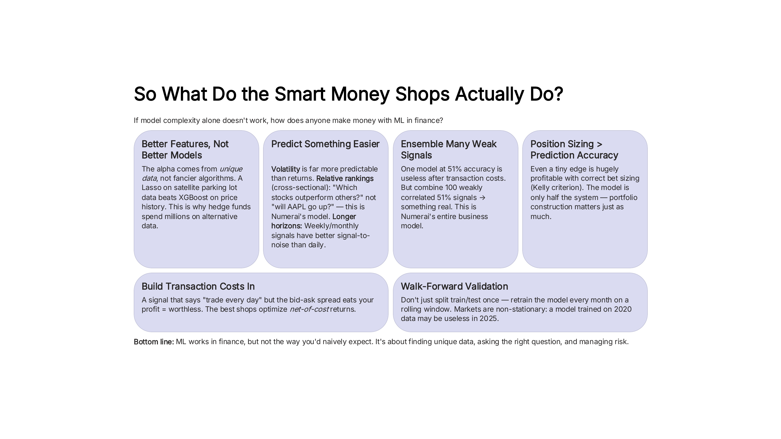
Fig. 95 How quantitative firms actually use ML in practice. Source: Professor Jonathan Hersh, BUS 696: Generative AI in Finance, Chapman University, Spring 2026.

Here are the key lessons:

Better features, not better models. The alpha comes from unique data, not fancier algorithms. A Lasso on satellite parking lot data beats XGBoost on price history. This is why hedge funds spend millions on alternative data.

Predict something easier. Volatility is far more predictable than returns. Relative rankings (cross-sectional: “which stocks outperform others?”) are easier than absolute predictions (“will AAPL go up?”). Longer horizons (weekly, monthly) have better signal-to-noise than daily.

Ensemble many weak signals. One model at 51% accuracy is useless after transaction costs. But combine 100 weakly correlated 51% signals, and you get something real. This is the business model behind firms like Numerai, which crowdsources signals from thousands of data scientists.

Build in transaction costs. A signal that says “trade every day” but the bid-ask spread eats your profit is worthless. The best shops optimize net-of-cost returns.

Walk-forward validation. Don’t just split train/test once. Retrain the model every month on a rolling window. Markets are non-stationary: a model trained on 2020 data may be useless in 2025.

Note

ML works in finance, but not the way you’d naively expect. It’s about finding unique data, asking the right question, and managing risk – not about finding the most complex model.

Position sizing > prediction accuracy

Perhaps the most surprising lesson from quantitative finance is this: how much you bet matters more than how often you’re right. This is where the Kelly Criterion comes in.

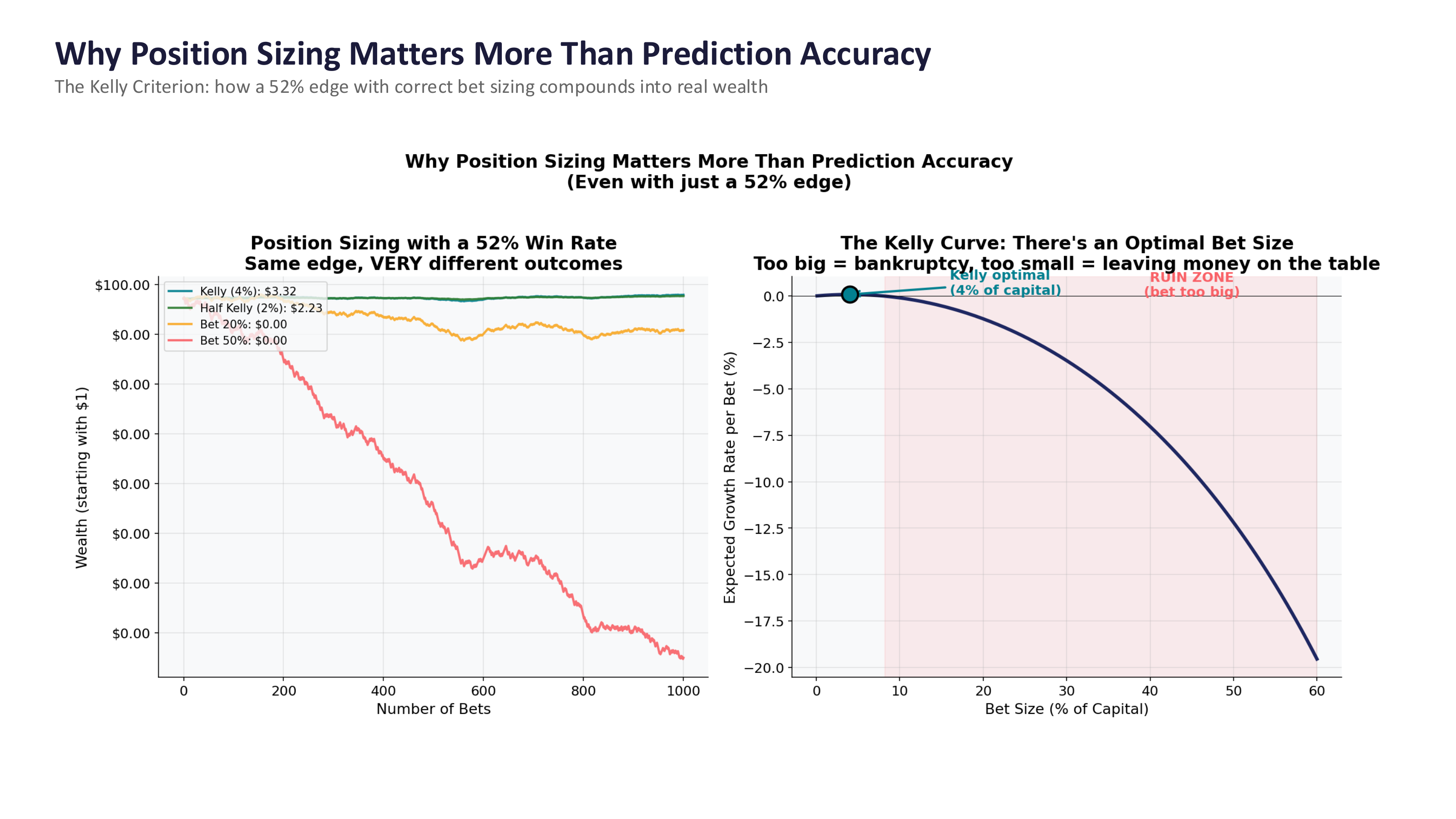
Fig. 96 Position sizing with a 52% win rate. Same edge, very different outcomes depending on bet size. The Kelly Criterion identifies the optimal bet size. Source: Professor Jonathan Hersh, BUS 696: Generative AI in Finance, Chapman University, Spring 2026.

The figure tells a powerful story. Both lines in the left panel start with the same 52% edge. But the Kelly-optimal strategy (betting ~4% of capital) grows steadily, while betting 20% or 50% of capital leads to ruin. The right panel shows the Kelly Curve – there is an optimal bet size, and betting too much is catastrophic.

The takeaway: the prediction model is only half the system. Portfolio construction – how you size positions, manage risk, and control for transaction costs – matters just as much, if not more. A mediocre model with excellent risk management will beat a great model with poor risk management every time.

Tip

This is why finance programs teach portfolio theory alongside data science. The prediction is just the input. What you do with that prediction – how you size the trade, when you exit, how you hedge – determines whether you make or lose money.